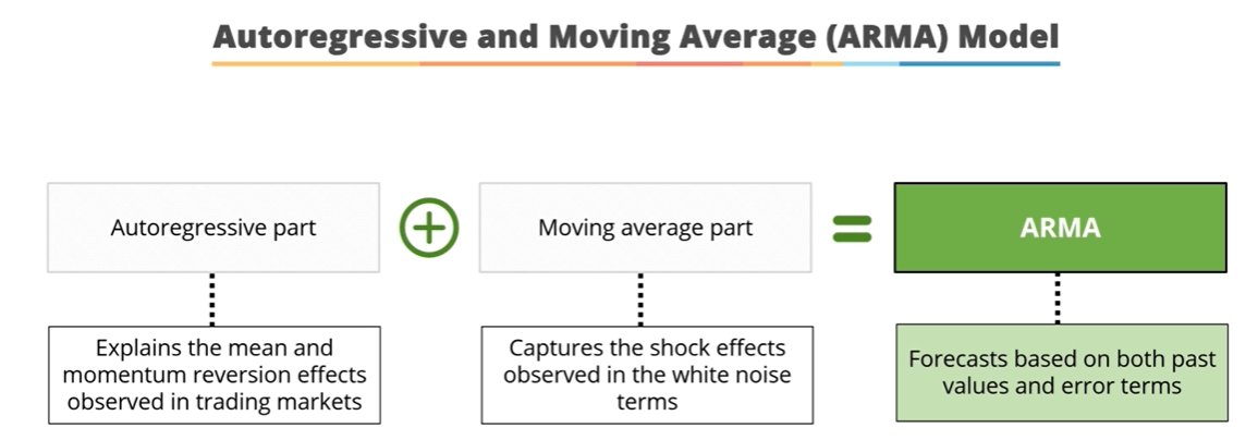
20.2 ACF and PACF for ARMA models
-The purpose is to identify the process underlying the data, which consists of identifying the \(p\) and $q orders of the ARMA model that generated the time series.
The tools to identify these processes are the simple (ACF) and partial (PACF) autocorrelation functions
Autocorrelation Function (ACF). The plot summarizes the correlation of an observation with lag values. The \(x\)-axis shows the lag and the \(y\)-axis shows the correlation coefficient between \(-1\) and \(1\) for negative and positive correlation.
Partial Autocorrelation Function (PACF). The plot summarizes the correlations for an observation with lag values that is not accounted for by prior lagged observations. Both plots are drawn as bar charts showing the 95% and 99% confidence intervals as horizontal lines. Bars that cross these confidence intervals are therefore more significant and worth noting.
- Correlograms only make sense within the scope of stationary processes because they assume that the correlation between two values in the series only depends on their distance, not on the instant of time to which they refer.
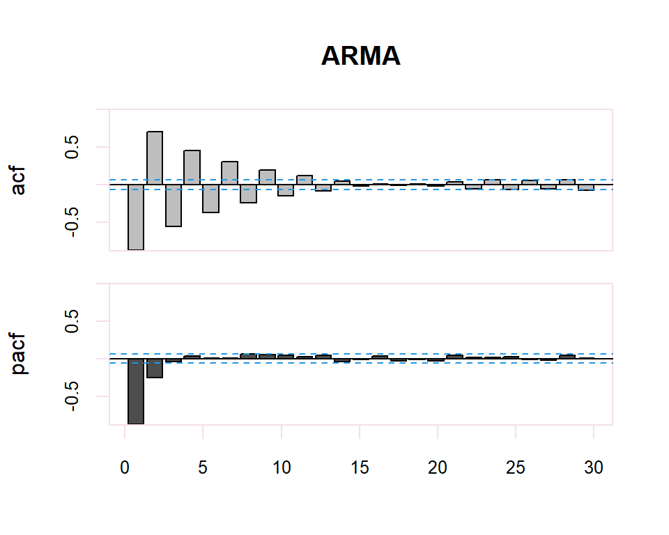
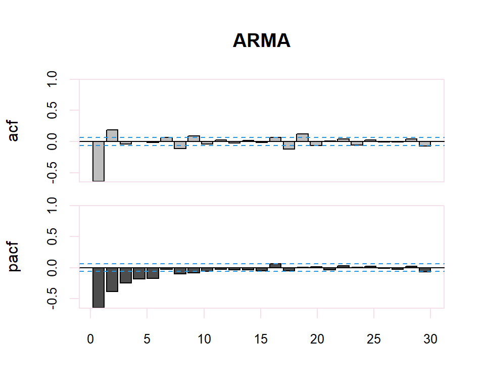
From these correlograms, the p and q orders of the corresponding ARMA model can be deduced. The duality between the AR and MA processes is again shown by the pattern of these models in both graphs.
Some useful patterns you may observe on these plots are:
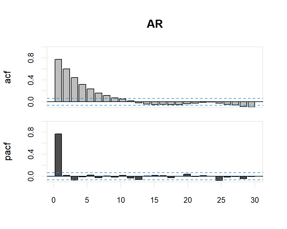
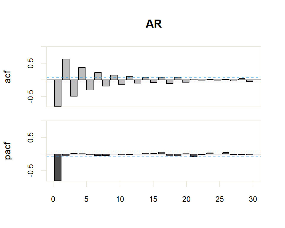
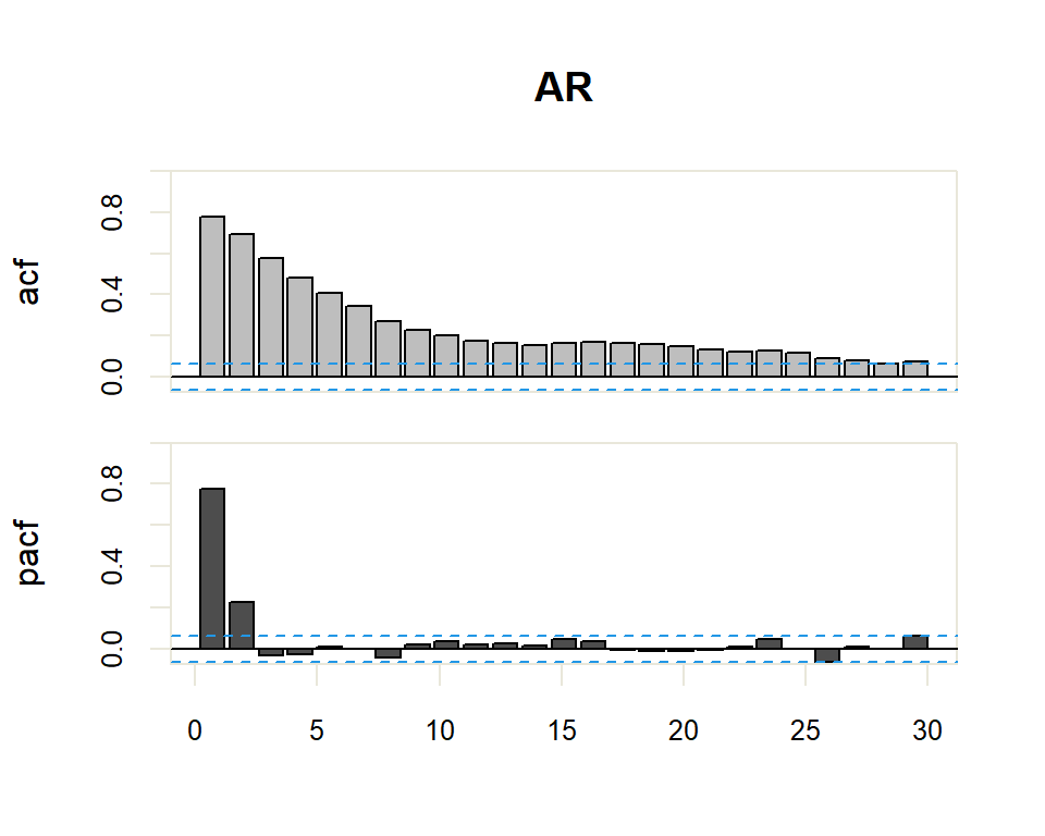
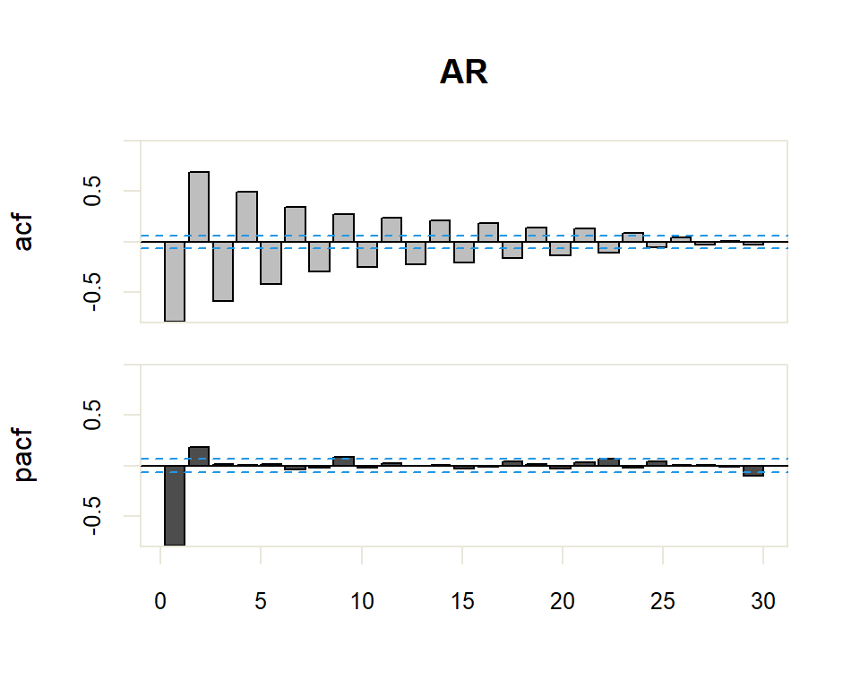
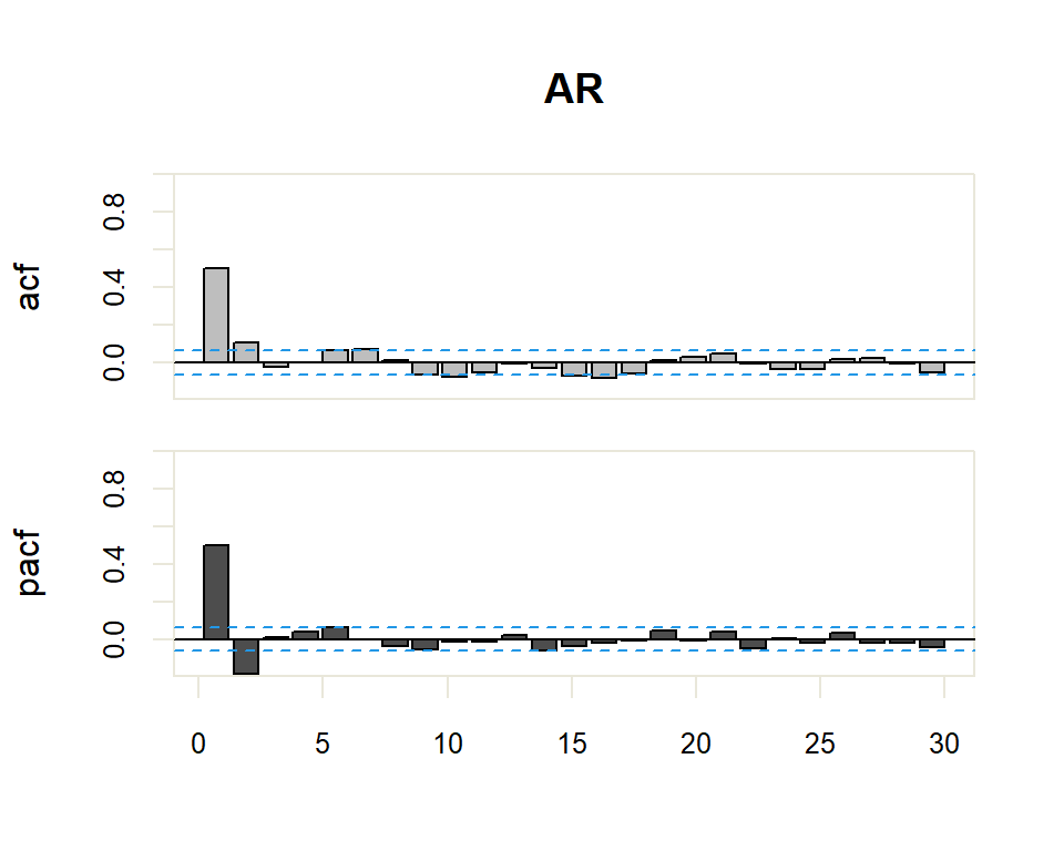
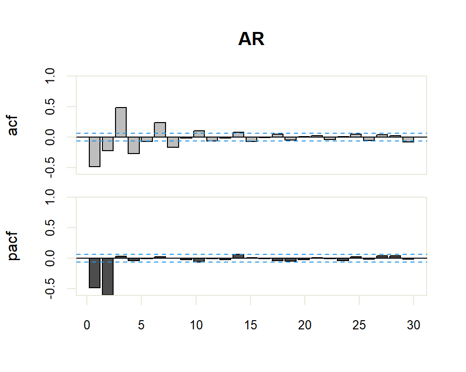
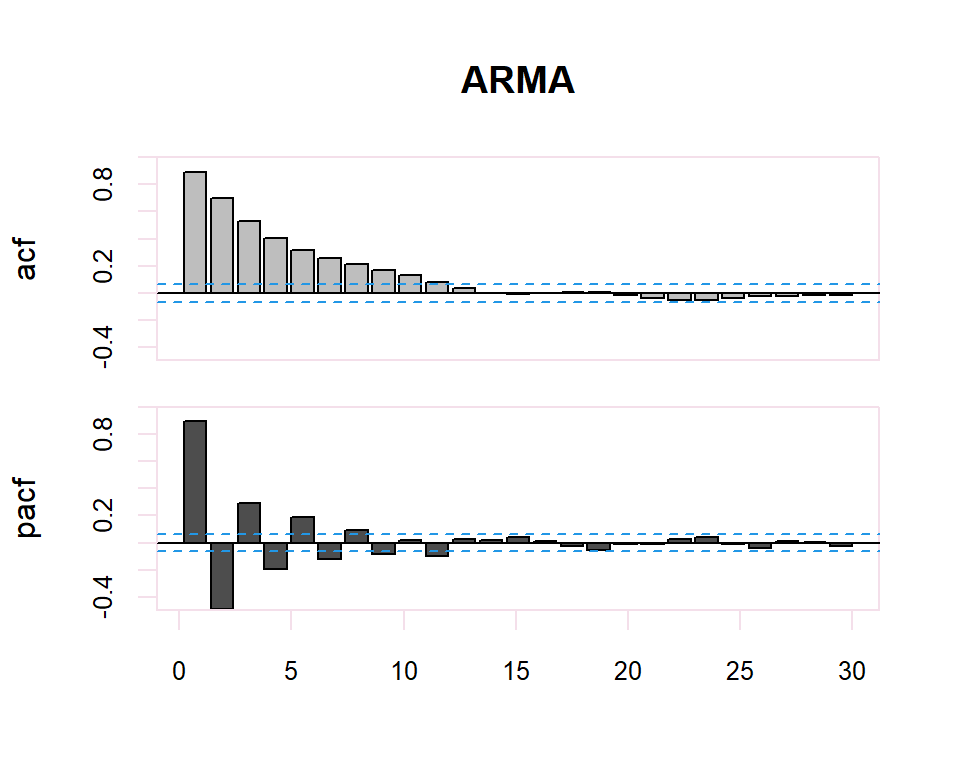
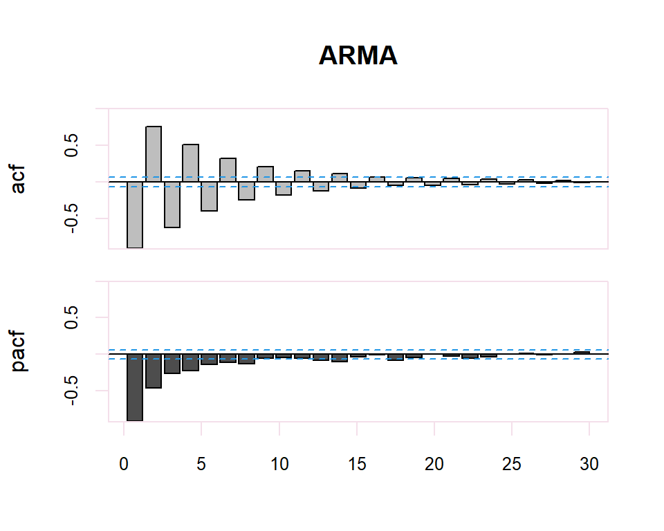
- The model is AR if the ACF trails off after a lag and has a hard cut-off in the PACF after a lag. This lag is taken as the value for \(p\).
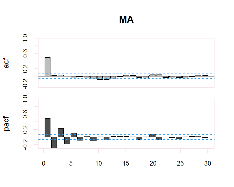
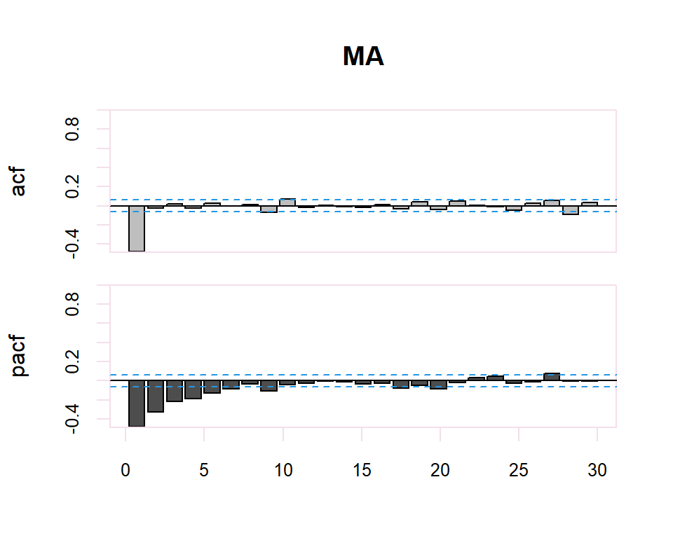
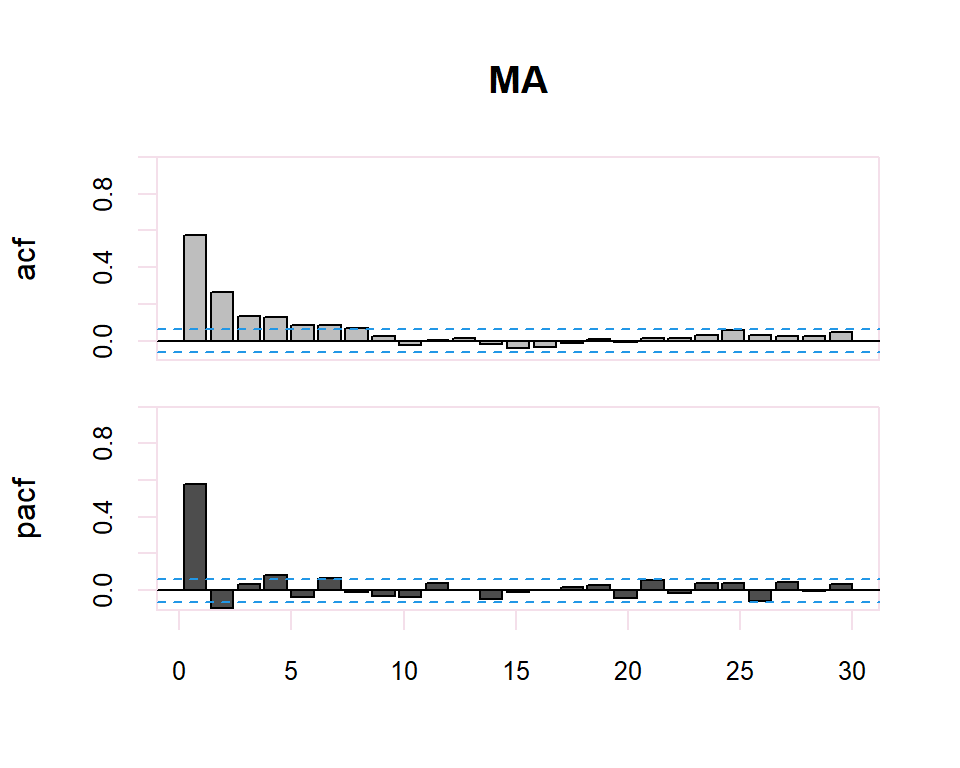
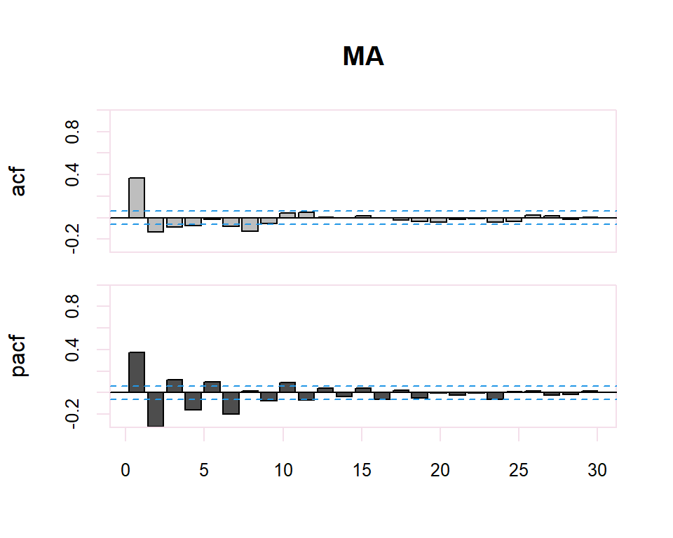
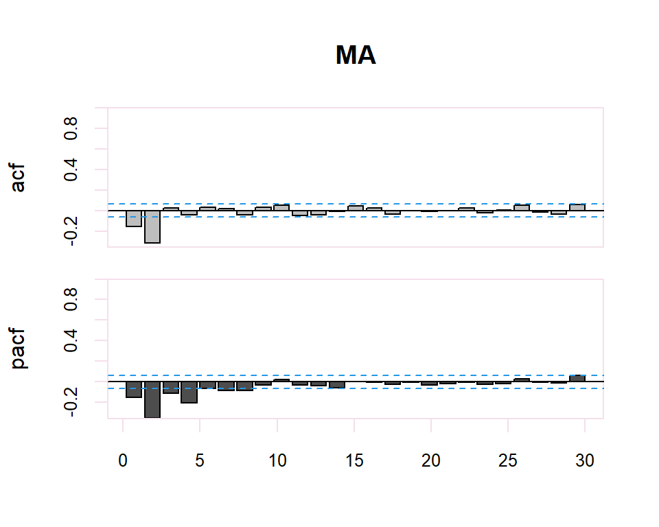
- The model is MA if the PACF trails off after a lag and has a hard cut-off in the ACF after the lag. This lag value is taken as the value for \(q\).
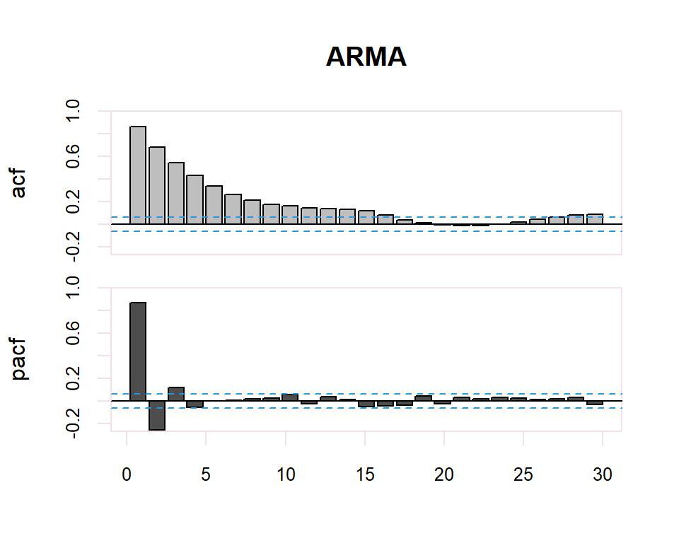
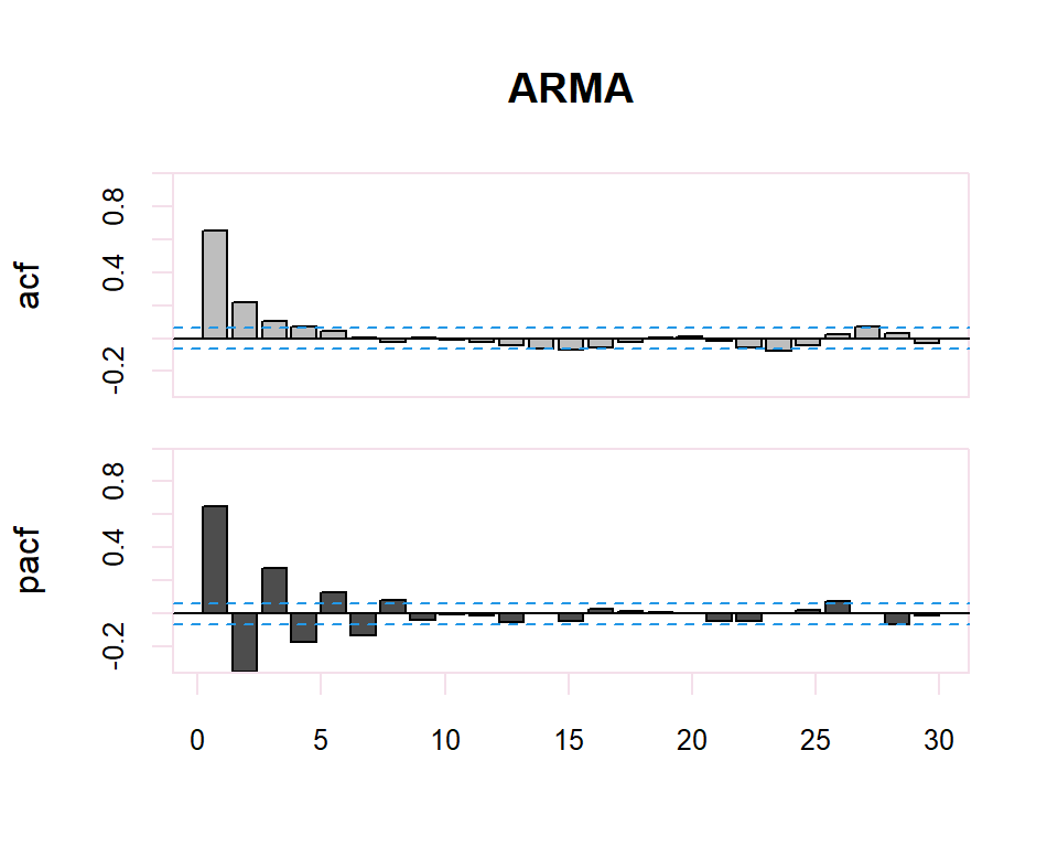
- The model is a mix of AR and MA if both the ACF and PACF trail off.
There is a duality between AR and MA processes, so that the PACF of an \(MA(q)\) has the structure of the ACF of an \(AR(q)\), and the ACF of an \(MA(q)\) has the structure of the PACF of an \(AR(q)\)

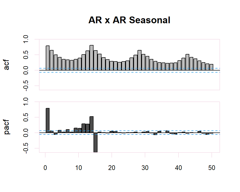
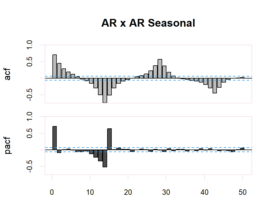
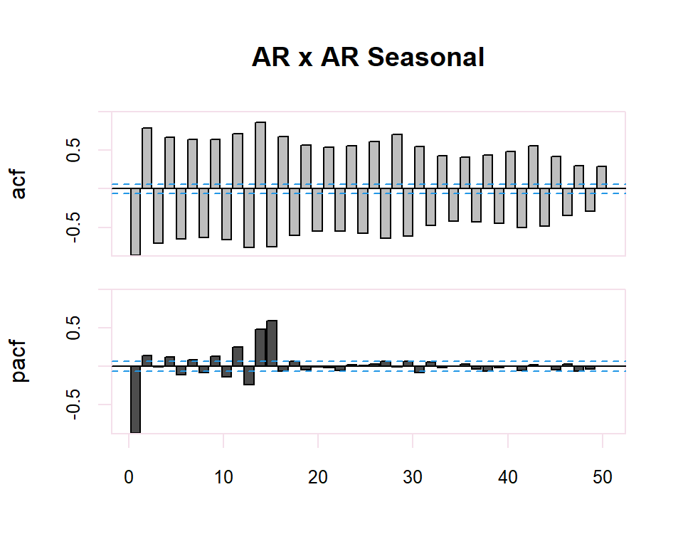
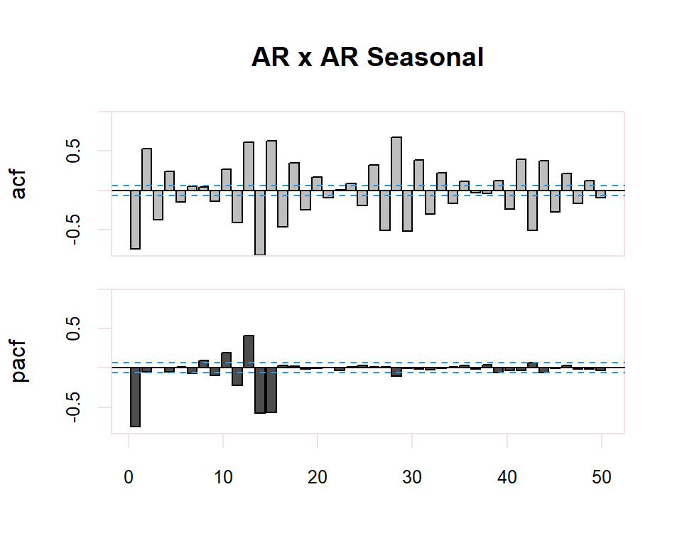
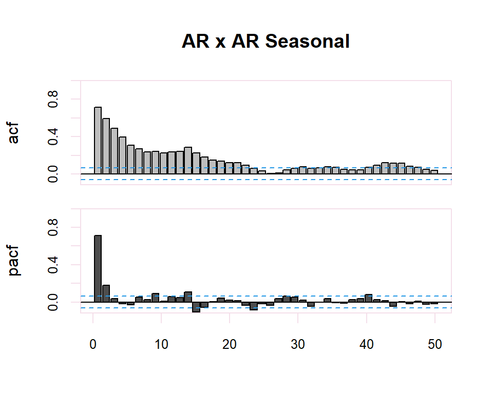
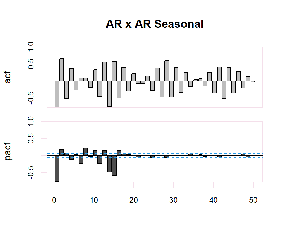
20.2.2 ARMA y ARMA Seasonal
| ACF | PACF | |
|---|---|---|
| \(AR(p)\) | Many non-zero coefficients (exponential and/or sinusoidal functions) | First \(p\) non-zero, rest 0 |
| \(MA(q)\) | First \(q\) non-zero, rest 0 | Many non-zero coefficients (exponential and/or sinusoidal functions) |
| \(ARMA (p,q)\) | Many non-zero coefficients (exponential and/or sinusoidal functions) | Many non-zero coefficients (exponential and/or sinusoidal functions) |
The identification process is totally subjective since it is a matter of determining whether the ACF or PACF decreases or is cutoff. However, tools are available to facilitate this task. For example, to determine whether the estimate of a simple or partial correlation coefficient is significantly different from zero a confidence region is available determined by the interval \({2}{N}\) where \(N\) is the number of observations in the series.
Finally, in the case of seasonality in the time series, the identification of the regular observed part of the time series will be performed. The identification of the regular part will be made by observing the first lags of the correlogram and of the seasonal part by observing the multiples of the observation frequency \(s\), of the series. In the seasonal case, the patterns of the previous table will also be followed. previous table will also be followed in the seasonal case.