7.5 Significancia de Parámetros

To determine whether the predictors introduced in a logistic regression model contribute significantly, the hypotheses must be tested:

\[ \begin{aligned} &H_{0}: \beta_{k}=0\\ &H_{1}: \beta_{k} \neq 0 \end{aligned} \] Fail to reject \(H_0\) would imply that there is insufficient evidence to claim that \(beta_k\) is different from zero. In other words, \(x_k\) is not statistically significant for the model in the presence of the remaining independent variables.

The Wald statistic is used to test these hypotheses.

\[W(\beta_k) = \dfrac{\hat\beta_k}{se(\hat\beta_k)},\]

where, if \(H_0\) is true, \(W(\beta_k)\) follows a Normal Distribution \(N(0,1)\) (also known as \(Z-\) test).

If the model has a single independent variable, the LLLR test can be used to evaluate \(H_0:\beta_1=0.\)

The confidence intervals for \(\beta_k\) can be estimated using a Normal Distribution. Thus an interval of \(100(1-\alpha)\) confidence for \(\beta_k\) is:

\[ \hat{\beta}_{k} \pm z_{\alpha / 2} se(\hat{\beta}_{k}) \]

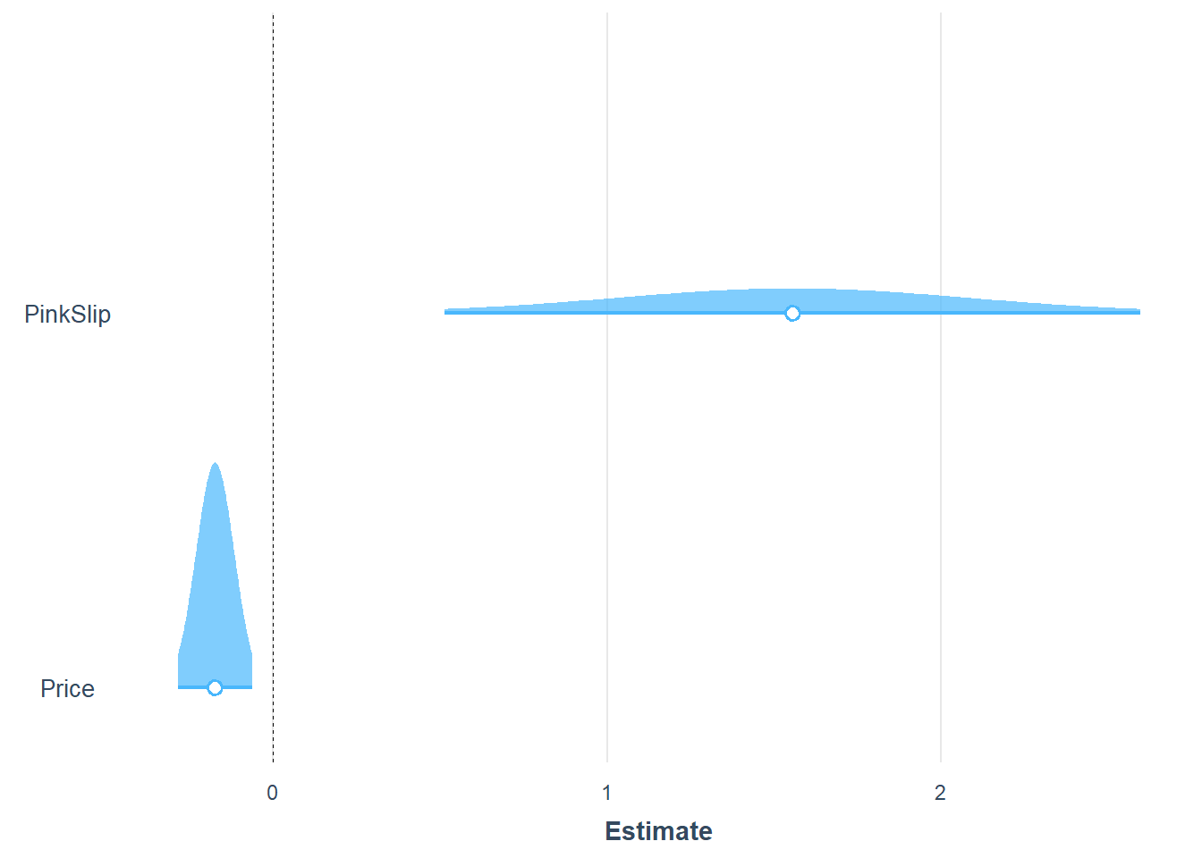
In our example:

\[ \log\left[ \frac { \widehat{P( \operatorname{Sold} = \operatorname{1} )} }{ 1 - \widehat{P( \operatorname{Sold} = \operatorname{1} )} } \right] = 0.4 - 0.17(\operatorname{Price}) + 1.55(\operatorname{PinkSlip}) \]

	Sold
Predictors	Odds Ratios	std. Error	Statistic	p
(Intercept)	1.49	0.71	0.82	0.410
Price	0.84	0.05	-3.04	0.002
PinkSlip	4.73	2.52	2.93	0.003
Observations	100
R² Tjur	0.185