17.3 ACF and PACF

In time series analysis, the objective is to identify the process underlying the data. The tools to identify these processes are the simple autocorrelation functions (ACF) and partial autocorrelation functions (PACF).

These functions are defined from the autocorrelation coefficients. They help to identify which observations contribute to the formation of the time series pattern.

The simple autocorrelation function (ACF) for a series gives correlations between the series $Y_{t}$ and lagged values of the series for lags of $1,2,3$, and so on. The lagged values can be written as $Y_{t-1}, Y_{t-2}, Y_{t-3}$, and so on. The ACF gives correlations between $Y_{t}$ and $Y_{t-1}, Y_{t}$ and $Y_{t-2}$, and so on.

The ACF can be used to identify the possible structure of time series data.

As a preliminary, we define an important concept, that of a stationary series. For an ACF to make sense, the series must be a weakly stationary series. This means that the autocorrelation for any particular lag is the same regardless of where we are in time

The simple autocorrelation function (ACF) can be estimated from the autocovariances of the process such that:

\[\hat \rho_{k}=\frac{\hat \gamma_k}{\hat \gamma_0}\]

where: \[\hat \gamma_0=\frac{\sum_{t=1}^{T}(Y_t-\bar Y)^2}{T}\] \[\hat \gamma_k=\frac{\sum_{t=k+1}^{T}(Y_t-\bar Y)(Y_{t+k}-\bar Y)}{T-k}\]

The partial autocorrelation function (PACF) measures the correlation between observations separated by $1, 2, \ldots, n$ periods, excluding the effect of intermediate correlations.

It should be taken into account that part of the simple correlation between the variable $Y$ at an instant $t$ and a previous instant $t-1$, may be due to the existing correlation of the variable with itself at intermediate instants.
For example, there may be some correlation between $Y_t$ and $Y_{t-2}$, because both variables are correlated with $Y_{t-1}$.

Considering AR(2):

\[ \begin{array}{r l} Y_t = & \phi_1 Y_{t-1}+\phi_2 Y_{t-2}\\ = & \phi_1 (\phi_1 Y_{t-2}+\phi_2 Y_{t-3})+\phi_2 Y_{t-2}\\ = & \phi_1^2 Y_{t-2} +\phi_2 Y_{t-2} + \phi_1 \phi_2 Y_{t-3} \end{array} \]

There is a direct effect of $Y_{t-2}$ on $Y_t$ through $Y_{t-2}$.
There is an indirect effect of $Y_{t-2}$ on $Y_t$ through $Y_{t-1},$ due to the fact that $Y_t$ and $Y_{t-1}$ are related by $\phi_1$.
If $\phi_1=0$, there would be no relationship between $Y_t$ and $Y_{t-1},$ so there would only be the direct effect between $Y_t$ and $Y_{t-2}.
There is a direct effect of $Y_{t-3}$ on $Y_t$ through $Y_{t-1}$ and $Y_{t-2}$.

The partial correlation between two variables in a set is the correlation after eliminating the effect of correlations with other variables. In other words, the PACF calculates the direct correlation by direct correlation by eliminating possible dependencies associated with intermediate lags

The correlogram is the graphical representation of the autocorrelation coefficients as a function of the different time series lags. They make it possible to represent the ACF and PACF functions.

A correlogram only makes sense in the realm of stationary processes because they assume that the correlation because they assume that the correlation between two values of the series only depends on their distance, not on the distance between them.

An example:

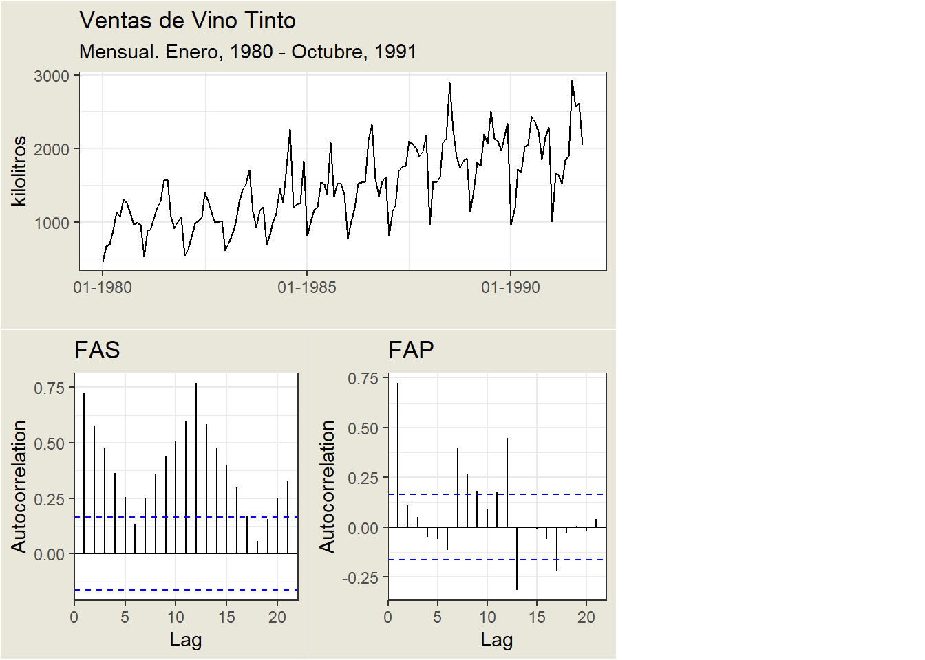
The $x$ axis of the ACF plot indicates the lag at which the autocorrelation is calculated; the $y$ axis indicates the value of the correlation (between -1 and 1).
For example, a peak at lag 1 of a ACF plot indicates that there is a strong correlation between the value of each series and the previous value, a peak at lag 2 indicates that there is a strong correlation between the value of each series and the value appearing two instants earlier, etc.
A positive correlation indicates that large current values correspond to large values at the specified lag; a negative correlation indicates that large current values correspond to small values at the specified lag.
The absolute value of a correlation is a measure of the strength of association, with larger absolute values indicating stronger relationships.