18.2 AR(1) properties
For an ACF to make sense, the series must be a weakly stationary series. This means that the autocorrelation for any given lag is the same regardless of where we are in time.
A time series \(Y_t\) is (weakly) stationary if it satisfies the following properties:
- \(E[Y_t]\) is the same for all \(t\)
- The Variance of \(Y_t\) is the same for all \(t\)
- The covariance (and correlation) between \(Y_t\) and \(Y_{t-1}\) is the same for all \(t\).
Let \(y_t\) be the value of a time series at time \(t\).
The ACF of a time series provides the correlation between \(y_t\) and \(y_{t-h}\) for \(h=1,2,3,\ldots\).
The (theoretical) autocorrelation between \(y_t\) and \(y_{t-h}\) is:
\[\dfrac{\text{Covariance}(y_t, y_{t-h})}{\text{Std.Dev.}(y_t)\text{Std.Dev.}(y_{t-h})} = \dfrac{\text{Covariance}(y_t, y_{t-h})}{\text{Variance}(y_t)} \]
\[ \rho_{h} = \frac{\sum\limits_{t=h+1}^T (y_{t}-\bar{y})(y_{t-h}-\bar{y})} {\sum\limits_{t=1}^T (y_{t}-\bar{y})^2}, \]
The denominator is the variance because the standard deviation of a stationary series is the same at all times. That is \(text{Std.Dev.}(y_t) = \text{Std.Dev.}(y_{t-h}), \forall h\).
The last property of a (weakly) stationary series says that the theoretical value of the autocorrelation of a given lag is the same throughout the series. An interesting property of a stationary series is that it theoretically has the same forward and backward structure.
Many stationary series have recognizable ACF patterns. However, most series we encounter in practice are non-stationary.
A continuous upward trend, for example, is a violation of the requirement that the mean be the same for the entire series. Distinct seasonal patterns also violate that requirement. Therefore, it is quite common to apply techniques to deal with non-stationary series.
18.2.1 Properties of AR(1)
An AR(1) is:
\[\begin{equation} y_t=\delta + \phi_1 y_{t-1}+\omega_t \end{equation}\]
The assumptions that must be met are:
- \(\omega_t\) are independent and are distributed as \(N(0,\sigma^2_\omega).\) The errors follow a Normal distribution with zero mean and constant variance.
- The properties of \(\omega_t\) are independent of \(y\).
- The series \(y_1, y_2, \ldots\) is (weakly) stationary.$ In the case of AR(1) this assumption implies that $|phi_1|<1.
The formulas for the mean, variance and ACF of a time series following an AR(1) process are:
- Mean \(y_t\)
\[\begin{equation} E(y_t)=\mu = \dfrac{\delta}{1-\phi_1} \end{equation}\]
- Variance \(y_t\)
\[\begin{equation} \text{Var}(y_t) = \dfrac{\sigma^2_w}{1-\phi_1^2} \end{equation}\]
- The correlation between observations separated by \(h\) periods of time is
\[\begin{equation} \rho_h = \phi^h_1 \end{equation}\]
\(\rho_h\) defines the theoretical ACF for time series with an AR(1) model .
\(\phi_1\) is the slope in the AR(1) model and is also the autocorrelation of lag 1.
18.2.2 AR(1)- ACF
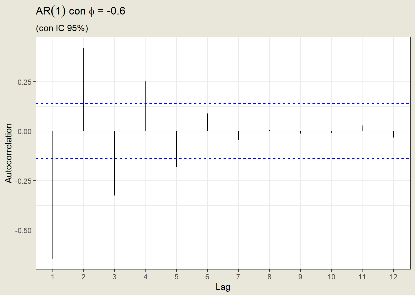
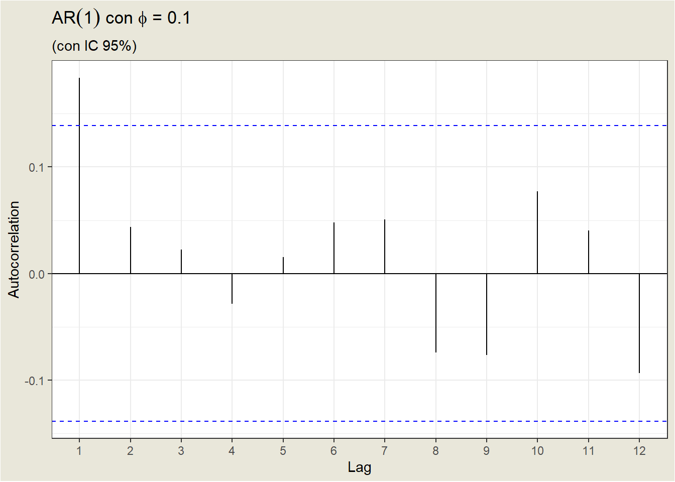
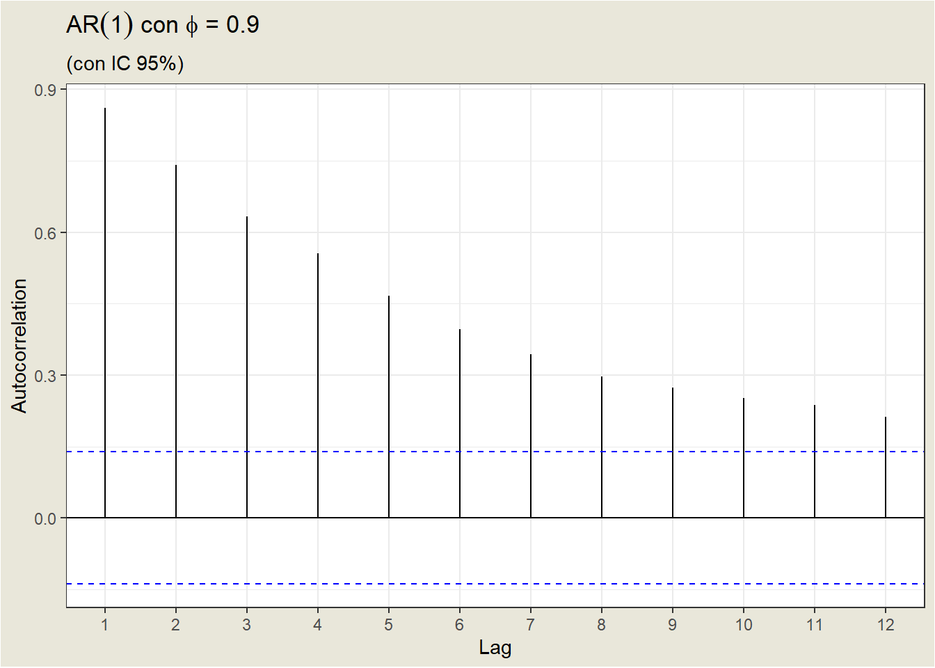
Depending on the value of \(phi_1\), the ACF defines a different pattern for the autocorrelations.
- For a positive value of \(phi_1\), the ACF decreases exponentially to 0 as the delay increases
- For a negative value of \(\phi_1\), the ACF also decays exponentially to 0 as the delay increases, but the signs of the autocorrelations alternate between positive and negative.
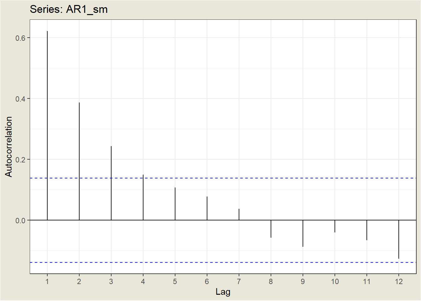
Let’s look at the ACF of the Earthquakes case:
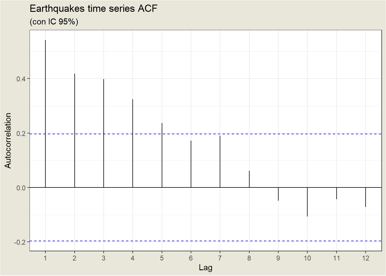
| Lag | 0 | 1 | 2 | 3 | 4 | 5 | 6 | 7 | 8 |
| ACF | 1.0000 | 0.5417 | 0.4189 | 0.3980 | 0.3240 | 0.2372 | 0.1718 | 0.1902 | 0.0612 |
Sampling autocorrelations decrease, but not as fast as expected for an AR(1). For example, theoretically, the autocorrelation of lag 2 for an AR(1) is the square of the autocorrelation of lag 1. In the example, \(\rho_2=\) 0.41888 when \(\rho_1^2=\) 0.2934714.
This case is an example of what happens in practice: the sample ACF rarely fits a perfect theoretical model. In most cases you have to try several models and choose the one that best fits the data.