18.1 AR(1)

The AR(1) model is

$$y_t=\delta + \phi_1 y_{t-1}+\omega_t$$

Assumptions:

• $\omega_{t} \stackrel{i i d}{\sim} N\left(0, \sigma_{\omega}^{2}\right)$, meaning that the errors are independently distributed with a normal distribution that has mean 0 and constant variance.
• Properties of the errors $\omega_{t}$ are independent of $y$.

	Observation
Parameter	Estimates	std. Error	t-test	p-value
(Intercept)	9.19	1.82	5.05	<0.001
lag1	0.54	0.09	6.37	<0.001
Observations	98
R2 / R2 adjusted	0.297 / 0.290

We see that the slope coefficient is significantly different from 0 , so the lag 1 variable is a helpful predictor. The $R^{2}$ value is relatively weak at $29.7 \%$, though, so the model won’t give us great predictions.

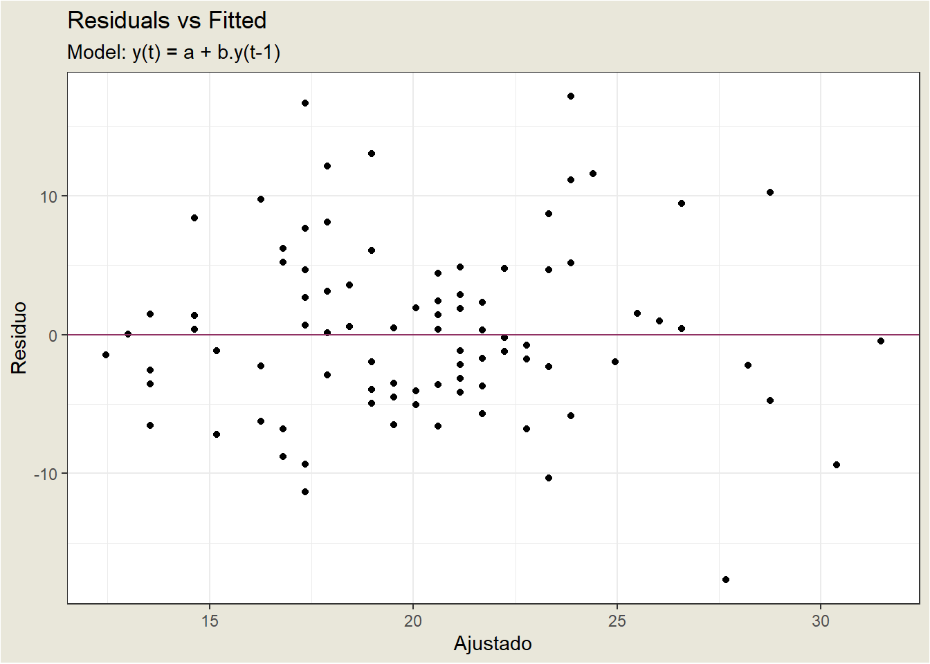
18.1.1 Residual Analysis

Continuing with the diagnosis, look at the plot of residuals versus fitted values. The ideal for this plot is to obtain a horizontal band of points. Below is a plot of the residuals versus the predicted values for our estimated model. It does not show any serious problems, except for a possible outlier at observation 28.

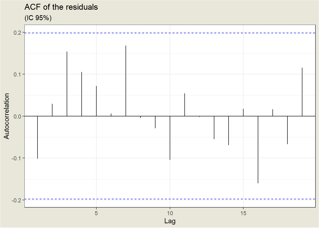
18.1.2 Sample Autocorrelation Function (ACF)

The sample autocorrelation function (ACF) for a series gives correlations between the series $y_{t}$ and lagged values of the series for lags of $1,2,3$, and so on. The lagged values can be written as $y_{t-1}, y_{t-2}, y_{t-3}$, and so on. The ACF gives correlations between $y_{t}$ and $y_{t-1}, y_{t}$ and $y_{t-2}$, and so on.

The ACF can be used to identify the possible structure of time series data.

The ACF of the residuals of a model is also useful. Ideally, the ACF of the residuals should show no significant correlations for any lag.

The ACF of the residuals for the earthquake example, where we use an AR(1) model, is shown below. The lag (time interval between observations) is shown on the horizontal axis, and the autocorrelation on the vertical axis. The horizontal lines indicate the limits of statistical significance. We can say that the ACF of the residuals is good since no correlation is significant; what we need for the residuals.