20.1 Box-Jenkins Method
The Box-Jenkins method was proposed by George Box and Gwilym Jenkins in their seminal 1970 textbook Time Series Analysis: Forecasting and Control.
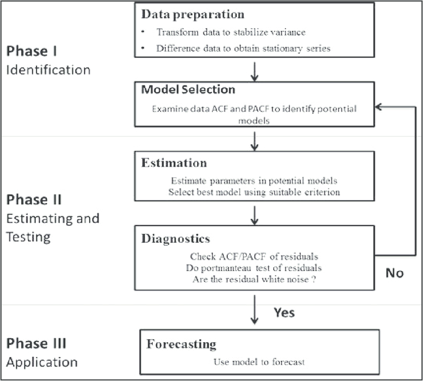
The approach starts with the assumption that the process that generated the time series can be approximated using an ARMA model if it is stationary or an ARIMA model if it is non-stationary.
The process of modeling is an iterative approach that consists of the following 3 steps:
- Identification. Use the data and all related information to help select a sub-class of model that may best summarize the data.
- Estimation. Use the data to train the parameters of the model (i.e. the coefficients).
- Diagnostic Checking. Evaluate the fitted model in the context of the available data and check for areas where the model may be improved.
It is an iterative process, so that as new information is gained during diagnostics, you can circle back to step 1 and incorporate that into new model classes.
20.1.1 Identification
The identification step is further broken down into:
- Assess whether the time series is stationary, and if not, how many differences are required to make it stationary.
- Identify the parameters of an ARMA model for the data.
20.1.2 Estimation
Estimation involves using numerical methods to minimize a loss or error term.
We will not go into the details of estimating model parameters as these details are handled by the chosen library or tool (Grtel).
20.1.3 Diagnostic Checking
The idea of diagnostic checking is to look for evidence that the model is not a good fit for the data.
Two useful areas to investigate diagnostics are:
- Overfitting
- Residual Errors.
20.1.3.1 Overfitting
The first check is to check whether the model overfits the data. Generally, this means that the model is more complex than it needs to be and captures random noise in the training data.
This is a problem for time series forecasting because it negatively impacts the ability of the model to generalize, resulting in poor forecast performance on out of sample data.
Careful attention must be paid to both in-sample and out-of-sample performance and this requires the careful design of a robust test harness for evaluating models.
20.1.3.2 Residual Errors
Forecast residuals provide a great opportunity for diagnostics.
A review of the distribution of errors can help tease out bias in the model. The errors from an ideal model would resemble white noise, that is a Gaussian distribution with a mean of zero and a symmetrical variance.
For this, you may use density plots, histograms, and Q-Q plots that compare the distribution of errors to the expected distribution. A non-Gaussian distribution may suggest an opportunity for data pre-processing. A skew in the distribution or a non-zero mean may suggest a bias in forecasts that may be correct.
Additionally, an ideal model would leave no temporal structure in the time series of forecast residuals. These can be checked by creating ACF and PACF plots of the residual error time series.
The presence of serial correlation in the residual errors suggests further opportunity for using this information in the model.
Forecasting: once the model is found to be valid, it is exploited, e.g. to forecast the analyzed series. This step can also be used in the diagnosis phase to select the “best” model.