6.2 Car Sales
![]()
| Variable | Descripción | Valores |
|---|---|---|
| Car ID | Identification code | 1 - 100 |
| Price | Sale Price of the car | 000s Eur |
| Age | Age of the car, | months |
| PinkSlip | Certificate of Title | 1: No, 2: Yes |
| Sold | Car sold? | 1: No, 2: Yes |
| Car ID | 1 | 2 | 3 | 4 | 5 | 6 | 7 | 8 | 9 | 10 | 11 | 12 |
| Price | 1 | 9 | 0 | 3 | 10 | 2 | 4 | 2 | 2 | 5 | 5 | 2 |
| Odometer | 30 | 20 | 170 | 68 | 12 | 88 | 3 | 41 | 21 | 74 | 41 | 121 |
| Age | 28 | 40 | 58 | 12 | 3 | 23 | 4 | 13 | 5 | 10 | 62 | 20 |
| PinkSlip | 1 | 1 | 0 | 1 | 0 | 0 | 1 | 1 | 1 | 1 | 0 | 1 |
| Sold | 1 | 0 | 1 | 1 | 0 | 0 | 0 | 1 | 1 | 1 | 0 | 1 |
| Nota: http://www.zstatistics.com/ |
The dataset:
| No | Variable | Stats / Values | Freqs (% of Valid) | Graph | Missing |
|---|---|---|---|---|---|
| 1 | Car ID [integer] |
Mean (sd) : 50.5 (29) min < med < max: 1 < 50.5 < 100 IQR (CV) : 49.5 (0.6) |
100 distinct values (Integer sequence) |
 |
0 (0.0%) |
| 2 | Price [numeric] |
Mean (sd) : 5.2 (5.1) min < med < max: 0.5 < 4 < 34.5 IQR (CV) : 5.5 (1) |
29 distinct values |  |
0 (0.0%) |
| 3 | Odometer [numeric] |
Mean (sd) : 60.1 (76.7) min < med < max: 0.2 < 30.5 < 452.5 IQR (CV) : 63 (1.3) |
100 distinct values |  |
0 (0.0%) |
| 4 | Age [integer] |
Mean (sd) : 20.2 (16.1) min < med < max: 1 < 15 < 90 IQR (CV) : 19 (0.8) |
39 distinct values |  |
0 (0.0%) |
| 5 | PinkSlip [integer] |
Min : 0 Mean : 0.8 Max : 1 |
0 : 23 (23.0%) 1 : 77 (77.0%) |
 |
0 (0.0%) |
| 6 | Sold [integer] |
Min : 0 Mean : 0.7 Max : 1 |
0 : 35 (35.0%) 1 : 65 (65.0%) |
 |
0 (0.0%) |
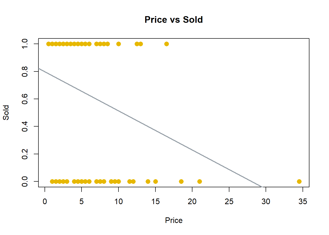 \[
\operatorname{\widehat{Sold}} = 0.8 - 0.03(\operatorname{Price})
\]
\[
\operatorname{\widehat{Sold}} = 0.8 - 0.03(\operatorname{Price})
\]
Let’s think of the fitted line as estimating the chance of being sold:
\[{\pi_i= Prob(\operatorname{Sold}=1)} = \beta_0 + \beta_1 \operatorname{Price}_i + \epsilon_i\]
What would be the probability of being sold of a car costing 45k euros? -> We need to transform/modify the dependent variable.
\[\dfrac{\pi_i}{1-\pi_i}={\dfrac{Prob(\operatorname{Sold}=1)}{1- Prob(\operatorname{Sold}=1)}} = \beta_0 +\beta_1 \operatorname{Price}_i + \epsilon_i\]
Evitamos obtener probabilidad negativa, la distribución es muy asimétrica (no Normal) -> Necesitamos transformar/modificar la variable dependiente.
Using logs:
\[\log \Bigl ( \dfrac{\pi_i}{1-\pi_i} \Bigr ) =\log \Bigl ( \dfrac{Prob(\operatorname{Sold}=1)}{1- Prob(\operatorname{Sold}=1)} \Bigr ) = \beta_0 +\beta_1\operatorname{Price}_i + \epsilon_i \]
The Binomial Logistic Regression is given by
\[\operatorname{logit}(\pi_i)= \log \Bigl ( \dfrac{\pi_i}{1-\pi_i} \Bigr ) = \beta_0 +\beta_1x_{1i}+\ldots+\beta_kx_{ki}\]
A model used to predict the probability of a certain class, given a set of independent variables.
-
Binomial: la variable dependiente es binaria, \(\pi_i = Prob(y_i=1)\)
-
Logistic: uses log-odds and the logit function
-
\(\beta_0, \beta_1, \ldots, \beta_k\) are the parameters
-
\(x_1, \ldots, x_k\) are the independent variables or predictors
Foe example:
\[\log \Bigl ( \dfrac{\pi_i}{1-\pi_i} \Bigr ) = \operatorname{logit} \Bigl [ Prob(\operatorname{Sold}=1) \Bigr ] = \beta_0 +\beta_1\operatorname{Price}_i\]
| Observations | 100 |
| Dependent variable | Sold |
| Type | Generalized linear model |
| Family | binomial |
| Link | logit |
| χ²(1) | 9.454 |
| Pseudo-R² (Cragg-Uhler) | 0.124 |
| Pseudo-R² (McFadden) | 0.073 |
| AIC | 124.036 |
| BIC | 129.246 |
| Est. | S.E. | z val. | p | |
|---|---|---|---|---|
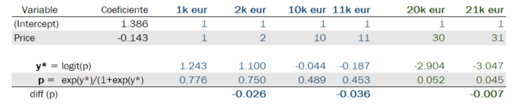
| (Intercept) | 1.386 | 0.356 | 3.894 | 0.000 |
| Price | -0.143 | 0.053 | -2.695 | 0.007 |
| Standard errors: MLE |
\[ \log\left[ \frac { \widehat{P( \operatorname{Sold} = \operatorname{1} )} }{ 1 - \widehat{P( \operatorname{Sold} = \operatorname{1} )} } \right] = 1.39 - 0.14(\operatorname{Price}) \]
What does -0.143 mean in the estimated model?
\[\widehat{\operatorname{logit}(\pi_i)} =1.386 -0.143 \operatorname{Price}_i\]
-
For each unit increase in \(\operatorname{Price}\), \(\operatorname{logit}(\pi)\) decreases in 0.143 units
-
What about \(\pi\)?
From \(\operatorname{logit}(\pi_i)\) to \(\pi_i\):
- we have:
\[ \operatorname{logit}(\pi) = \log \Bigl ( \dfrac{\pi}{1-\pi} \Bigr )=\beta_0 +\beta_1 \operatorname{Price}\]
- then:
\[\pi = \dfrac{e^{\beta_0 +\beta_1 \operatorname{Price}}}{1+e^{\beta_0 +\beta_1 \operatorname{Price}}}\] - O alternativamente (más fácil):
\[\pi = \dfrac{e^{\operatorname{logit}(\pi) }}{1+e^{\operatorname{logit}(\pi) }}\]
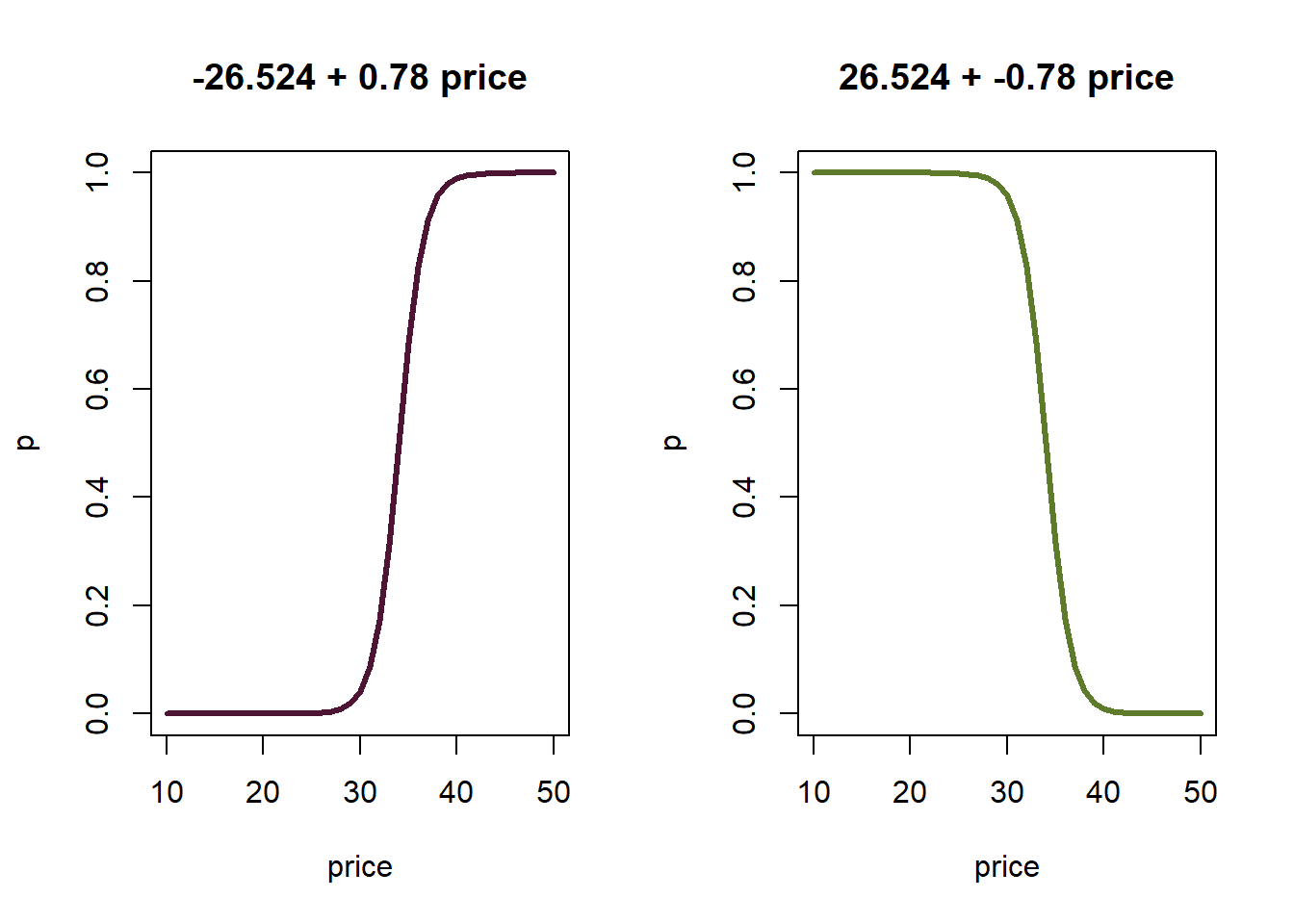
In the example:
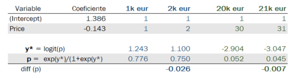
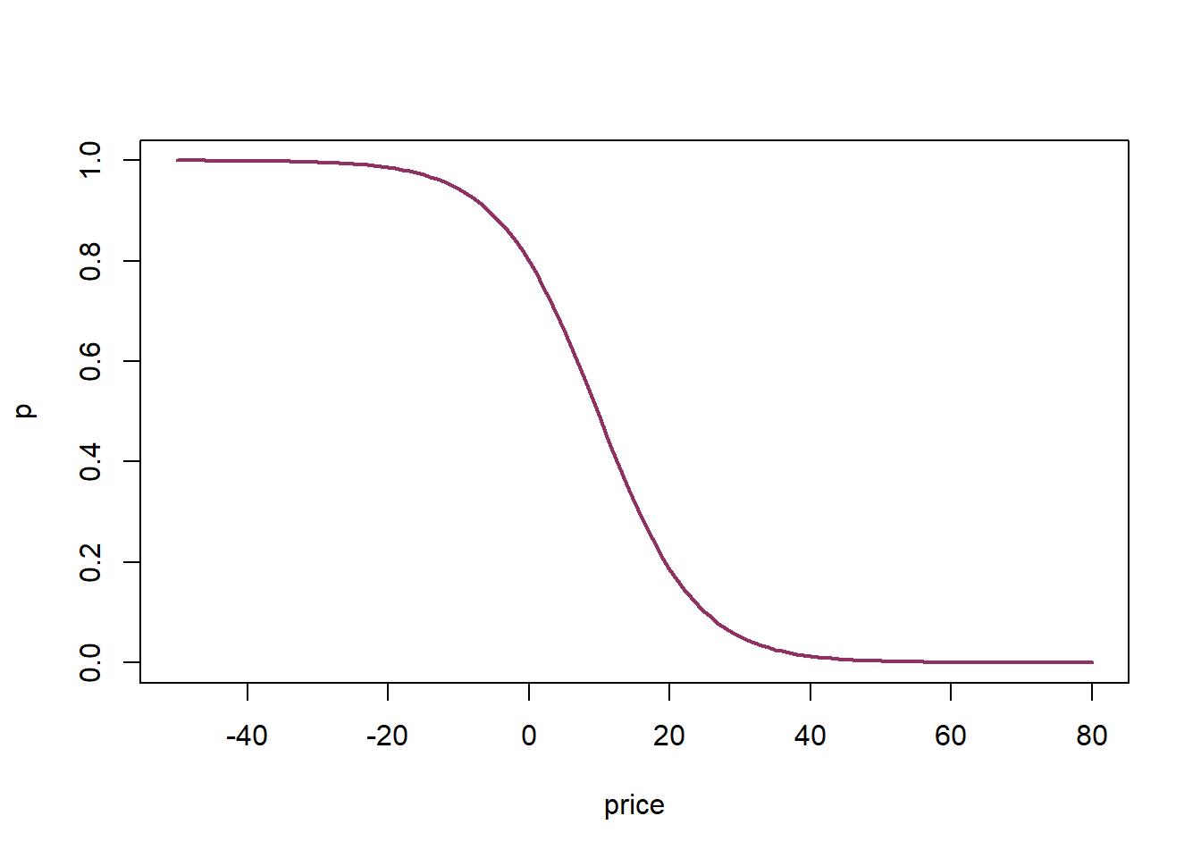
The coefficients determine the curve:
Multiple Logistic Regression
Assume that the \(operatorname{logit}\) transformation of the dependent variable has a linear relationship with a set of independent variables.
Let us include one more variable in the model.
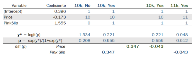
\[\log \Bigl ( \dfrac{\pi_i}{1-\pi_i} \Bigr ) =\log \Bigl ( \dfrac{Prob(\operatorname{Sold_i}=1)}{1- Prob(\operatorname{Sold_i}=1)} \Bigr ) = \beta_0 +\beta_1\operatorname{Price}_i +\beta_2\operatorname{Pink Slip}_i\]
| Observations | 100 |
| Dependent variable | Sold |
| Type | Generalized linear model |
| Family | binomial |
| Link | logit |
| χ²(2) | 18.407 |
| Pseudo-R² (Cragg-Uhler) | 0.232 |
| Pseudo-R² (McFadden) | 0.142 |
| AIC | 117.083 |
| BIC | 124.898 |
| Est. | S.E. | z val. | p | |
|---|---|---|---|---|
| (Intercept) | 0.396 | 0.480 | 0.824 | 0.410 |
| Price | -0.173 | 0.057 | -3.044 | 0.002 |
| PinkSlip | 1.555 | 0.531 | 2.926 | 0.003 |
| Standard errors: MLE |
\[ \log\left[ \frac { \widehat{P( \operatorname{Sold} = \operatorname{1} )} }{ 1 - \widehat{P( \operatorname{Sold} = \operatorname{1} )} } \right] = 0.4 - 0.17(\operatorname{Price}) + 1.55(\operatorname{PinkSlip}) \]
Let’s estimate \(\pi\)
Parameter’s interpretation:
The coefficients of the logistic regression estimate the change in log-odds of the dependent variable given a one-unit increase in the independent variable.
| Coeficiente | 2.5 % | 97.5 % | |
|---|---|---|---|
| (Intercept) | 0.396 | -0.552 | 1.354 |
| Price | -0.173 | -0.295 | -0.071 |
| PinkSlip | 1.555 | 0.533 | 2.632 |
\(\beta_1=-0.173\) : If the price increases by 1000 euros, the log-odds of selling the car decreases, in mean, by 0.173, holding the rest constant.
\(\beta_2= 1.555\) : If the car has Pink Slip, the log-odds of selling the car increase, on average, by 1,555, holding the rest constant.
If we apply $exp to the coefficients, we can interpret them as odds-ratios.
| OR | 2.5 % | 97.5 % | |
|---|---|---|---|
| (Intercept) | 1.486 | 0.576 | 3.872 |
| Price | 0.841 | 0.745 | 0.931 |
| PinkSlip | 4.734 | 1.704 | 13.903 |
\(\exp(\beta_1)=0.84\): If Price increases by one unit, the odds of being sold (versus not being sold) increases by a factor of 0.84.
\(\exp(\beta_2)=4.73\): If Pink Slip increases by one unit, the odds of being sold (vs. not being sold) increase by a factor of 4.73.
-
\(\beta\) represents the effect of \(x\) on log-odds.
-
\(\operatorname{exp}(\beta)\) represents the effect of \(x\) on odds-ratio.