6.1 Coronary Heart Disease (CHD)
![]()
It is of interest to explore the relationship between age and the presence or absence of CHD in a population.
We have the age in years (AGE) and the presence or absence of evidence of significant heart disease (CHD) for 100 subjects selected to participate in a study. The outcome variable is CHD, which is coded with a value of zero to indicate CHD is absent, or 1 to indicate that it is present in the individual.
| Variable | Description | Values |
|---|---|---|
| ID | Identification code | 1 - 100 |
| AGE | Age | Years |
| AGE_GROUP | Age group | 1: 20-39, 2: 30-34, 3: 35-39, 4: 40-44, 5: 45-49, 6: 50-54, 7: 55-59, 8: 60-69 |
| CHD | Presence of CHD | 1: No, 2: Yes |
Fuente: David W. Hosmer Jr., Stanley Lemeshow, Rodney X. Sturdivant (2013). Applied Logistic Regression, 3rd Edition. ISBN: 978-0-470-58247-3. 528 Pages.
The first 12 datapoint in the sample are:
| 1 | 2 | 3 | 4 | 5 | 6 | 7 | 8 | 9 | 10 | 11 | 12 | |
|---|---|---|---|---|---|---|---|---|---|---|---|---|
| ID | 1 | 2 | 3 | 4 | 5 | 6 | 7 | 8 | 9 | 10 | 11 | 12 |
| AGE | 20 | 23 | 24 | 25 | 25 | 26 | 26 | 28 | 28 | 29 | 30 | 30 |
| AGE_GROUP | 20-39 | 20-39 | 20-39 | 20-39 | 20-39 | 20-39 | 20-39 | 20-39 | 20-39 | 20-39 | 30-34 | 30-34 |
| CHD | No | No | No | No | Yes | No | No | No | No | No | No | No |
| Fuente: https://rdrr.io/cran/aplore3/man/chdage.html |
Descriptive analysis of the dataset:
| No | Variable | Stats / Values | Freqs (% of Valid) | Graph | Missing |
|---|---|---|---|---|---|
| 1 | ID [integer] |
Mean (sd) : 50.5 (29) min < med < max: 1 < 50.5 < 100 IQR (CV) : 49.5 (0.6) |
100 distinct values (Integer sequence) |
 |
0 (0.0%) |
| 2 | AGE [integer] |
Mean (sd) : 44.4 (11.7) min < med < max: 20 < 44 < 69 IQR (CV) : 20.2 (0.3) |
43 distinct values |  |
0 (0.0%) |
| 3 | AGE_GROUP [factor] |
1. 20-39 2. 30-34 3. 35-39 4. 40-44 5. 45-49 6. 50-54 7. 55-59 8. 60-69 |
10 (10.0%) 15 (15.0%) 12 (12.0%) 15 (15.0%) 13 (13.0%) 8 ( 8.0%) 17 (17.0%) 10 (10.0%) |
 |
0 (0.0%) |
| 4 | CHD [factor] |
1. No 2. Yes |
57 (57.0%) 43 (43.0%) |
 |
0 (0.0%) |
How is the relationaship between CHD and AGE?
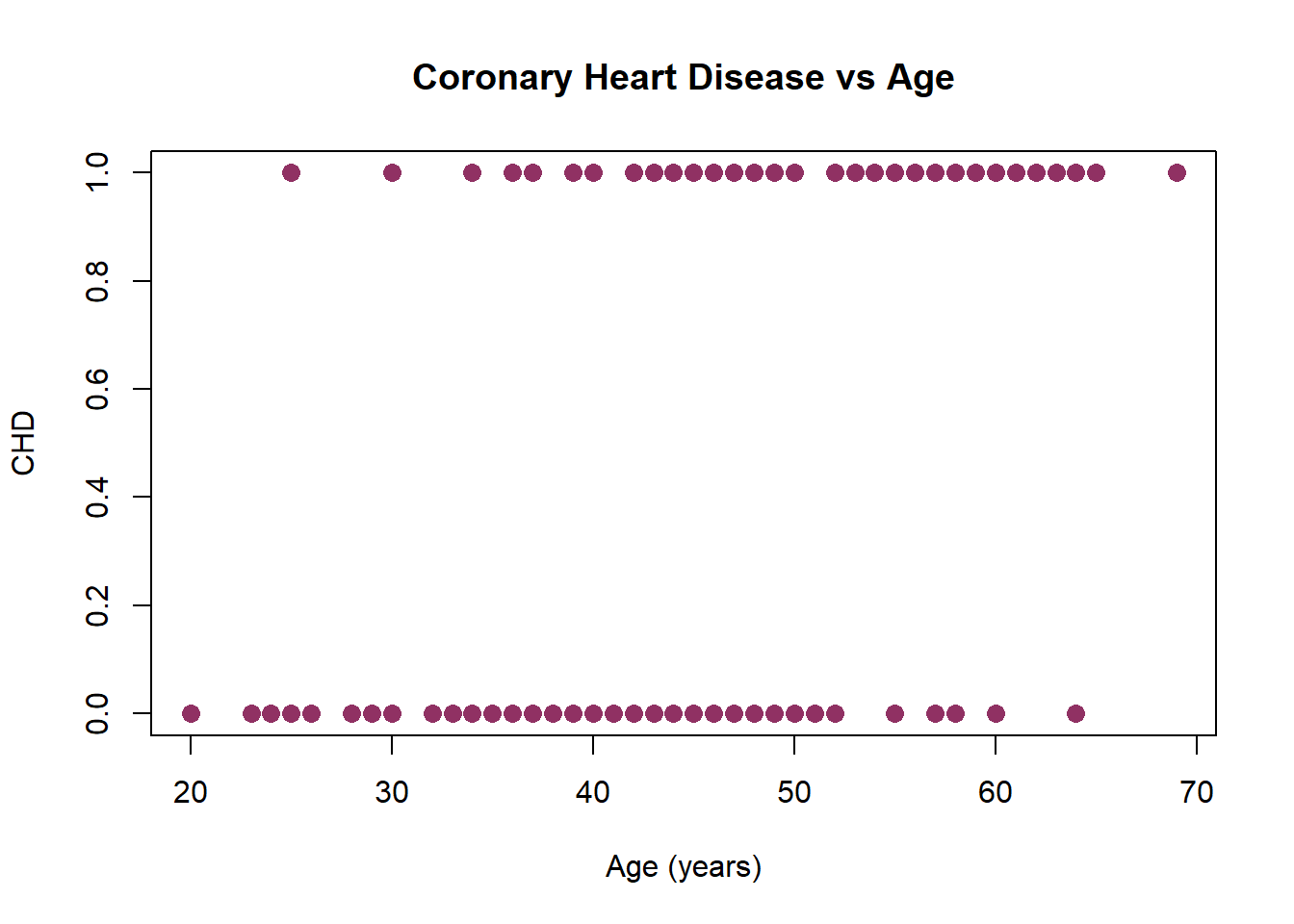
In the scatterplot of CHD by AGE for 100 subjects (below) all points fall on one of two parallel lines representing the absence of CHD (\(y=0\)) and the presence of CHD (\(y=1\)). There is some tendency for the individuals with no evidence of CHD to be younger than those with evidence of CHD.
Can we use a simple linear regression?
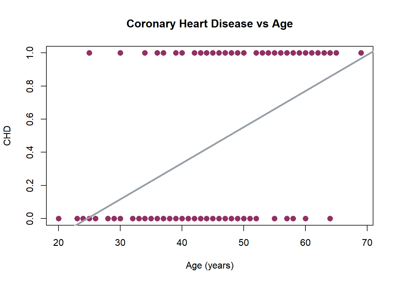 \[
\operatorname{\widehat{CHD\_}} = -0.54 + 0.02(\operatorname{AGE})
\]
\[
\operatorname{\widehat{CHD\_}} = -0.54 + 0.02(\operatorname{AGE})
\]
Let’s create intervals for the independent variable AGE and compute the mean of the outcome variable CHD within each group. The new age group variable is AGE_GROUP. In the table below we have the frequency of occurrence of each outcome as well as the mean (or proportion with CHD present) for each age group.
| CHD:No | CHD:Yes | n | p | |
|---|---|---|---|---|
| 20-39 | 9 | 1 | 10 | 0.10 |
| 30-34 | 13 | 2 | 15 | 0.13 |
| 35-39 | 9 | 3 | 12 | 0.25 |
| 40-44 | 10 | 5 | 15 | 0.33 |
| 45-49 | 7 | 6 | 13 | 0.46 |
| 50-54 | 3 | 5 | 8 | 0.62 |
| 55-59 | 4 | 13 | 17 | 0.76 |
| 60-69 | 2 | 8 | 10 | 0.80 |
| Sum | 57 | 43 | 100 | 0.43 |
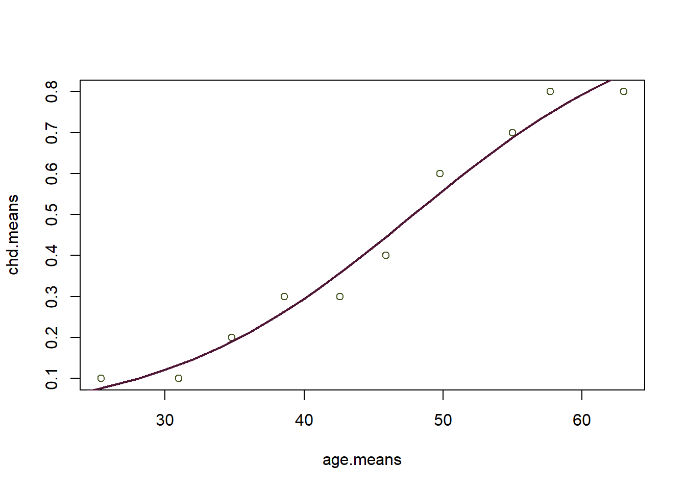
The plot of the proportion of individuals with CHD (CHD=Yes) versus the midpoint of each interval provides considerable insight into the relationship between CHD and age in this study. A functional form for this relationshio needs to be described.
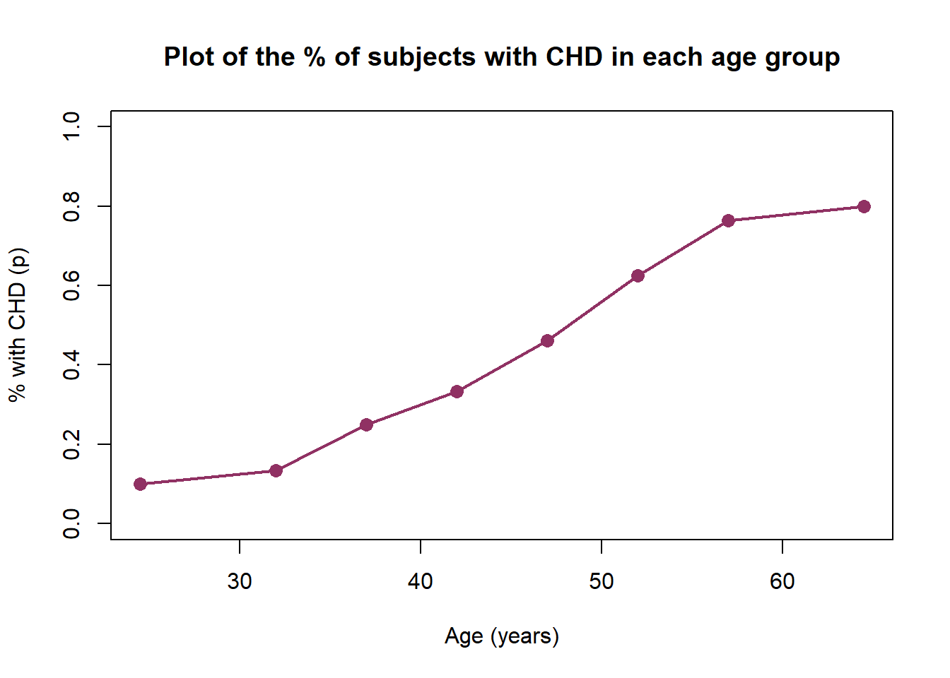
The curve represents \(E[Y|x]\), the “expected value of \(Y\), given the value \(x\)”. The plot shows that this mean approaches zero and 1 gradually. The change in the \(E[Y|x]\) per unit change in \(x\) becomes progressively smaller as the conditional means gets closer to zero or 1
The curve is said to be S-shaped. It resembles a plot of the cumulative distribution of a random variable.It should not seem surprising that some well-known cumulative distributions have been used to provide a model for \(E[Y|x]\) in the case when \(Y\) is dichotomous.
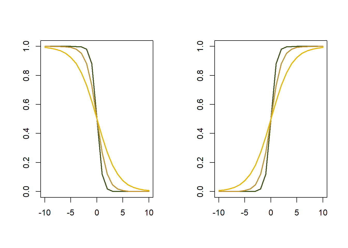
The logistic function can be used to model \(E[Y|x]\)
The logistic funtion or logistic curve is S-shaped and given by:
\[f(x)=\dfrac{L}{1+e^{-k(x-x_0)}}\] where
- \(x_0\) is the value of \(x\) in the midpoint of the curve
- \(L\) is the maximun
- \(k\) is the growth rate
Therefore, if
\[ y_i \sim \text{Bernoulli}(\pi_i) \]
where \(\pi_i\) is the probability of \(y_i=1\) and
\[ \pi_i = \dfrac{1}{1+e^{-(\beta_0+\beta_1x_i)}} \] Since \(0<\pi_i<1\), to assure taht \(E[Y|x]\) is a number between \(-\infty\) and \(+\infty\), we obtain \(1-p_i,\) the probability of \(y_i=0\):
\[ 1-\pi_i = \dfrac{e^{-(\beta_0+\beta_1x_i)}}{1+e^{-(\beta_0+\beta_1x_i)}} \] The odds (or ratio between probabilities) is \[ \dfrac{\pi_i}{1-\pi_i} = \dfrac{1}{e^{-(\beta_0+\beta_1x_i)}} \] Using \(\log\) to both sides:
\[ \log \Bigl( \dfrac{\pi_i}{1-\pi_i} \Bigr ) = \beta_0+\beta_1x_i \] is the equation of a simple linear regression model with dependent variable: \(\log ( \frac{\pi_i}{1-\pi_i})=\operatorname{logit}(\pi_i(x))\)
The fitted model is:
| Observations | 100 |
| Dependent variable | CHD |
| Type | Generalized linear model |
| Family | binomial |
| Link | logit |
| χ²(1) | 29.31 |
| Pseudo-R² (Cragg-Uhler) | 0.34 |
| Pseudo-R² (McFadden) | 0.21 |
| AIC | 111.35 |
| BIC | 116.56 |
| Est. | S.E. | z val. | p | |
|---|---|---|---|---|
| (Intercept) | -5.31 | 1.13 | -4.68 | 0.00 |
| AGE | 0.11 | 0.02 | 4.61 | 0.00 |
| Standard errors: MLE |
Remember that the coefficient estimates are for the transformed model. They provide a linear fit for \(\operatorname{logit}(\pi(x))\), not for \(\pi(x)\). However, if we define an inverse logit function, we can transform our model back to the original metric.
Below, we plot the mean AGE against the mean CHD for groups of 10 observations, then superimpose the logistic regression fit, transformed back into the probability metric
6.1.1 Interpreting Model Coefficients
6.1.1.1 Binary Predictor
Suppose there is a single predictor, and it is categorical (0,1). How can one interpret the coefficient \(\beta_1\)?
Consider the odds ratio, the ratio of the odds when \(x = 1\) to the odds when \(x = 0\).
According to our model, \(\operatorname{logit}(\pi(x)) = exp(\beta_0 + \beta_1 x)\), so the log of the odds ratio is given by
\[ \begin{aligned} \log (O R) &=\log \left[\frac{\pi(1) /(1-\pi(1))}{\pi(0) /(1-\pi(0))}\right] \\ &=\log \left [\frac{\pi(1)}{1-\pi(1)} \right ]-\log \left [ \frac{\pi(0)} {1-\pi(0)} \right] \\ &=\operatorname{logit}(\pi(1))-\operatorname{logit}(\pi(0)) \\ &=\beta_{0}+\beta_{1} \times 1-\left(\beta_{0}+\beta_{1} \times 0\right) \\ &=\beta_{1} \end{aligned} \] Exponentiating both sides, we get
\[OR = \exp(\beta_1)\] - Suppose that X represents the presence or absence of a medical treatment, and \(\beta_1 = 2\). This means that the odds ratio is \(\exp(2) = 7.389\). If the event is survival, this implies that the odds of surviving are \(7.389\) times as high when the treatment is present than when it is not.
- You can see why logistic regression is very popular in medical research, and why there is a tradition of working in the odds metric.
6.1.1.2 Continuous predictor
In our coronary heart disease data set, the predictor is continuous. Interpreting model coefficients when a predictor is continuous is more difficult.
Recalling the form of the fitted function for \(\pi(x)\), we see that it does not have a constant slope.
By taking derivatives, we compute the slope as \(\beta_1 \pi(x)(1 − \pi(x)).\) Hence, the steepest slope is at \(\pi(x) = 1/2\), at which \(x = −\beta_0/\beta_1\), and the actual slope is \(β_1/4\).
A note: in toxicology, this is called \(LD50\), because it is the dose at which the probability of death is \(1/2\).
So a rough rule of thumb is that when \(X\) is near the middle of its range, a unit change in \(X\) results in a change of \(\beta_1/4\) units in \(\pi(x)\).
In the CHD example, the estimated value of \(\beta_1\) is \(0.1069\), and the estimated value of \(\beta_0 is −5.1263\). This suggests that, around the age of \(45\), an increase of 1 year in AGE corresponds roughly to an increase of \(0.0267\) in the probability of coronary heart disease.
We will see that in the linear zone near the center of the plot, the rule of thumb works quite well. The rule implies that for every increase of 4 units in \(AGE\), there will be roughly a \(\beta_1\) increase in the probability of coronary heart disease.
| x | |
|---|---|
| 45 | 0.4211628 |
| 46 | 0.4484140 |
| 47 | 0.4759786 |
| 48 | 0.5036903 |
| 49 | 0.5313794 |
| 50 | 0.5588765 |
-
The method use is MLE (maximum likeñlihoo estimation) not MCO.
-
Parameters interpretation is different!.