4 Introduction
Logistic regression is applicable, for example, if we want to…
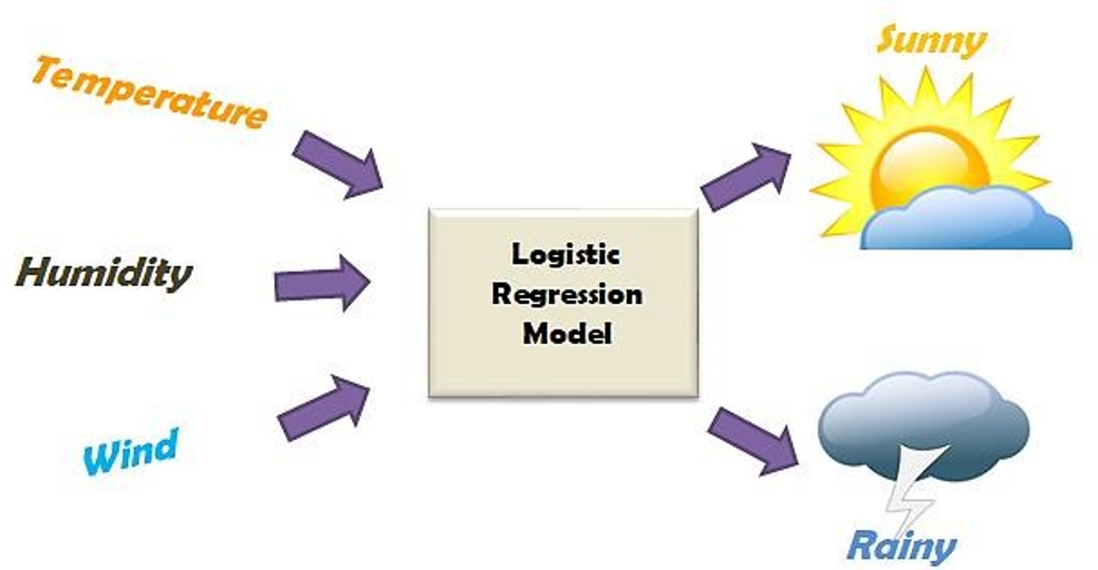
- model the probabilities of a response variable as a function of some explanatory variables, e.g., “success” of admission as a function of sex.
- perform descriptive discriminate analyses such as describing the differences between individuals in separate groups as a function of explanatory variables, e.g., student admitted and rejected as a function of sex.
- classify individuals into two categories based on explanatory variables, e.g., classify new students into “admitted” or “rejected” groups depending on sex.
As we’ll see, there are two key differences between binomial (or binary) logistic regression and classical linear regression:
- Instead of a normal distribution, the logistic regression response has a Bernoulli distribution (can be either “success” or “failure”), and
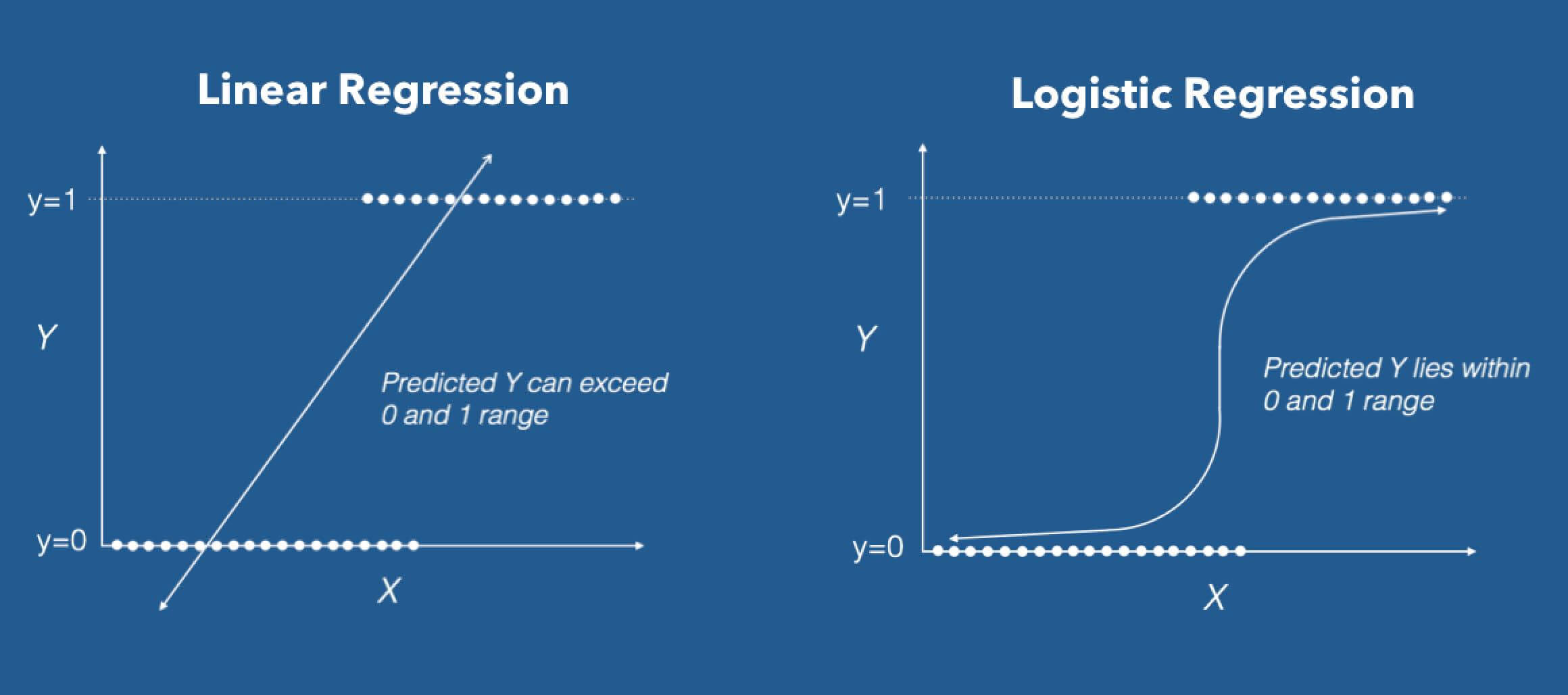
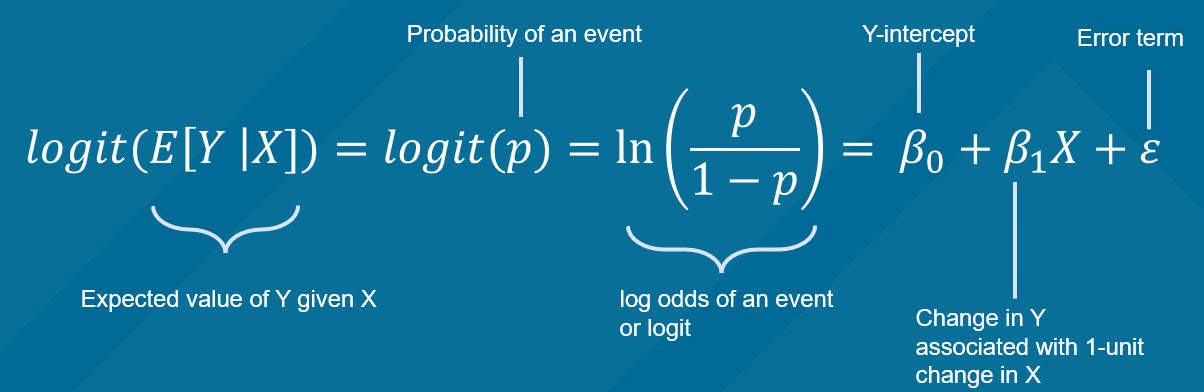
- Instead of relating the response directly to a set of predictors, the logistic model uses the log-odds of success—a transformation of the success probability called the logit. Among other benefits, working with the log-odds prevents any probability estimates to fall outside the range (0, 1).
The most basic of all discrete random variables is the Bernoulli. \(X\) is said to have a Bernoulli distribution if \(X=1\) occurs with probability \(\pi\) and \(X=0\) occurs with probability \(1-\pi\),
\[ f(x)=\left\{\begin{array}{ r l } \pi & x=1 \\ 1-\pi & x=0 \\ 0 & \text { otherwise } \end{array}\right. \] Another common way to write it is… \[ f(x)=\pi^{x}(1-\pi)^{1-x} \text { for } x=0,1 \] Suppose an experiment has only two possible outcomes, “success” and “failure,” and let \(\pi\) be the probability of a success. If we let \(X\) denote the number of successes (either zero or one), then \(X\) will be Bernoulli. The mean (or expected value) of a Bernoulli random variable is \[ E(X)=1(\pi)+0(1-\pi)=\pi, \] and the variance is… \[ V(X)=E\left(X^{2}\right)-[E(X)]^{2}=1^{2} \pi+0^{2}(1-\pi)-\pi^{2}=\pi(1-\pi) \]
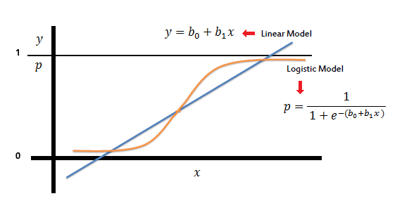
When \(f(X)\) is a simple linear regression: \(y_i = \beta_0 +\beta_1x_{i} +\epsilon_i\).
The expected value of the dependent variable \(Y,\) given the value of the independent variable \(x\) is given by \(E[Y|x]=\beta_0 +\beta_1x_{1}.\) Then \(E[Y|x] \in (-\infty,+\infty)\)
Fuente: Aquí
-
The sign of the estimated coefficient represents the direction of the influence of the independent variable on the dependent variable: positive or negative.
-
We can use the std.error to construct confidence intervals on the model parameters. Note that the \(N(0,1)\) distribution is used
-
The method use is MLE (maximum likeñlihoo estimation) not MCO.
-
Parameters interpretation is different!.