19.7 MA(1)

MA(1)

A stationary univariate stochastic process $(Y_t)$ follows a model MA(1) when

$$Y_t=\delta +\phi_1 Y_{t-1} + \phi_2 Y_{t-2}+\omega_t$$ where $ _t$ is a white noise with zero mean and variance $\sigma^2_\omega, \,\, \rightarrow \,\, \omega_t \sim N(0,\sigma^2_\omega).$

When a stationary process $\left(Y_{t}\right)$ follows a $\operatorname{MA}(1),$

$$Y_{t}=\mu+\omega_{t}-\theta_{1} \omega_{t-1}$$

with $\left|\theta_{1}\right|<1$ $\mathrm{y}\left(\omega_{t}\right) \sim \operatorname{IID}\left(0, \sigma_{\omega}^{2}\right)$, it can verified that:

• Mean:

$$\mu_{Y}=\mu$$

Since:

$$E[Y_t]=\mu + \underbrace{E[\omega_t]}_0+ \theta_1 \underbrace{E[\omega_{t-1}]}_0 = \mu$$

• Variance: $$\sigma_{Y}^{2}=\left(1+\theta_{1}^{2}\right) \sigma_{\omega}^{2}$$

given that:

$$\begin{aligned} \gamma_0 = Var(Y_t) &= E[(Y_t-\mu)^2] \\ &= E[(\omega_t+\theta_1\omega_{t-1})^2] \\ &= E[\omega_t^2+\theta_1^2\omega_{t-1}^2 + 2\theta_1\omega_{t}\omega_{t-1}]\\ &= \sigma^2_{\omega} + \theta_1^2\sigma^2_{\omega} + 2\theta_1 \underbrace{E[\omega_t\omega_{t-1}]}_0\\ &= (1+\theta_1^2)\sigma^2_{\omega} \end{aligned}$$

• Autocovariance:

$$\begin{aligned} \gamma_{1}=\operatorname{Cov}\left(Y_{t}, Y_{t-1}\right)&=E\left[\left(Y_{t}-\mu\right)\left(Y_{t-1}-\mu\right)\right]\\ &=E\left[\left(\omega_{t}+\theta_1 \omega_{t-1}\right)\left(\omega_{t-1}+\theta_1 \omega_{t-2}\right)\right] \\ &=E\left[\omega_{t} \omega_{t-1}+\theta_1 \omega_{t-1}^{2}+\theta_1 \omega_{t} \omega_{t-2}+\theta_{1}^{2} \omega_{t-1} \omega_{t-2}\right] \\ &=E\left[\omega_{t} \omega_{t-1}\right]+\theta_1 E\left[\omega_{t-1}^{2}\right]+\theta_1 E\left[\omega_{t} \omega_{t-2}\right]+\theta_{1}^{2} E\left[\omega_{t-1} \omega_{t-2}\right] \\ &=\theta_1 \sigma^{2}_\omega \end{aligned}$$

$$\begin{array}{l} \gamma_{2}=\operatorname{Cov}\left(Y_{t}, Y_{t-2}\right)&=E\left[\left(Y_{t}-\mu\right)\left(Y_{t-2}-\mu\right)\right] \\ \quad&=E\left[\left(\omega_{t}+\theta_1 \omega_{t-1}\right)\left(\omega_{t-2}+\theta_1 \omega_{t-3}\right)\right] \\ \quad&=E\left[\omega_{t} \omega_{t-2}+\theta_1 \omega_{t-1} \omega_{\ell-2}+\theta_1 \omega_{t} \omega_{t-3}+\theta_1^{2} \omega_{t-1} \omega_{t-3}\right] \\ \quad&=0 \end{array}$$

In general, for any lag $\geq 2,$

$$\gamma_{j}=\operatorname{Cov}\left(Y_{t}, Y_{t-j}\right)=E\left[\left(Y_{t}-\mu\right)\left(Y_{t-j}-\mu\right)\right]=0 \quad \forall j \geq 2$$

From these results we can obtain the autocorrelations.

• ACF:

$$\rho_{j}=\left\{\begin{array}{ll} 1 & \text { si } j=0 \\ \dfrac{\theta_{1}}{\left(1+\theta_{1}^{2}\right)} & \text { si } j=1 \\ 0 & \quad \forall j>1 \end{array}\right.$$

• PACF:

$$\phi_{jj}=-\left[\frac{1}{\sum_{i=0}^{j} \theta_{1}^{2 i}}\right] \theta_{1}^{j}=-\left[\frac{1-\theta_{1}^{2}}{1-\theta_{1}^{2(j+1)}}\right] \theta_{1}^{j} \quad \forall j \geq 1$$

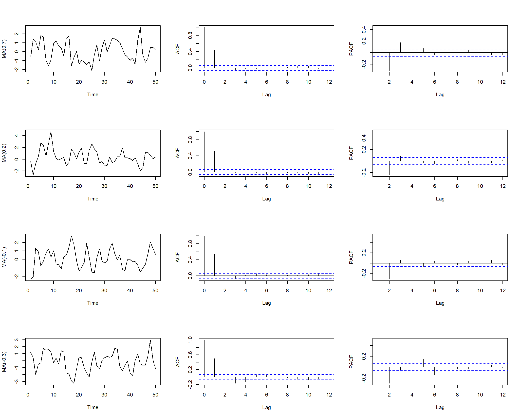
Examples:

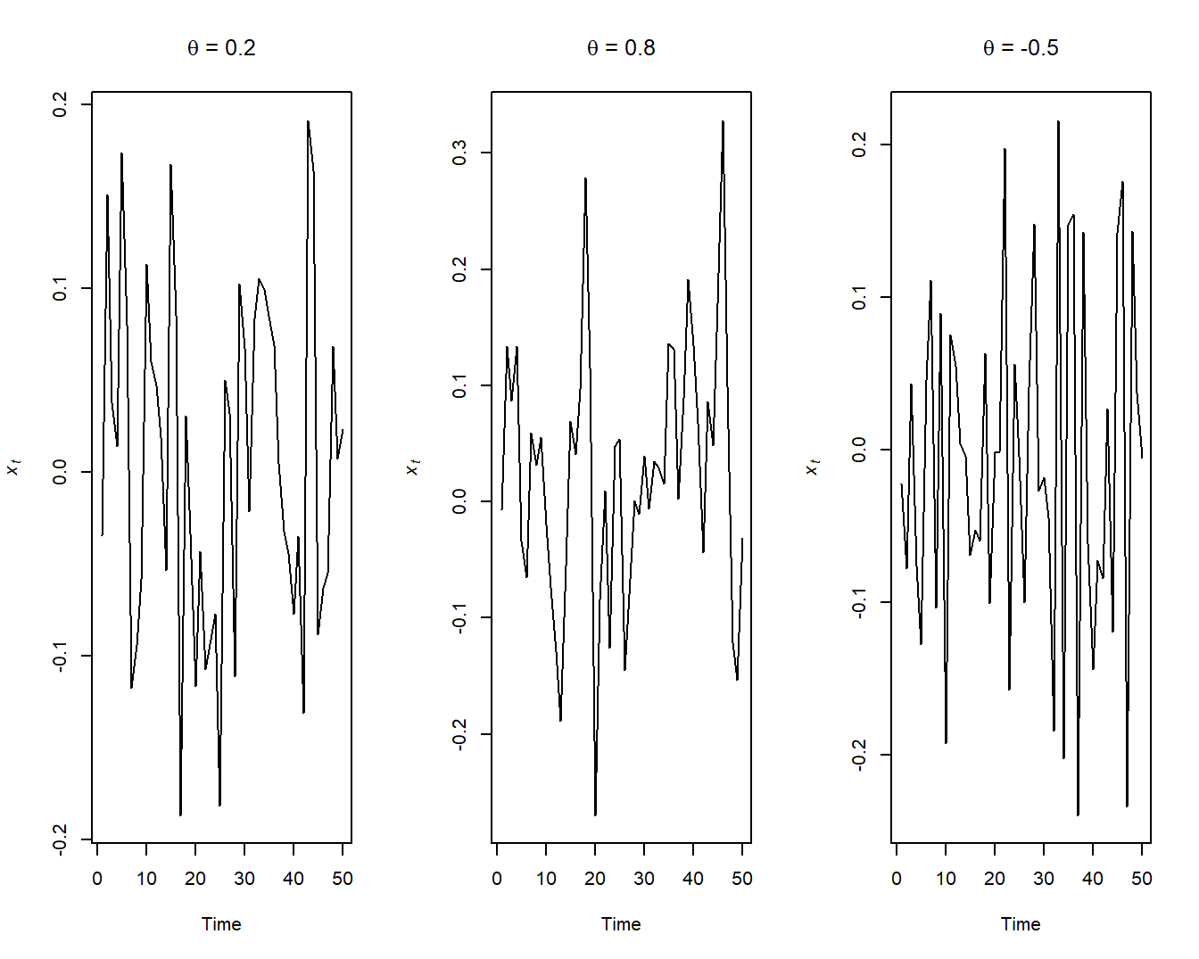
The MA(1) process has short memory