16.1 Moving-average models
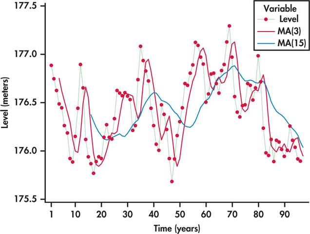
Perhaps the most common method used in practice to smooth out short-term fluctuations is the moving-average model. A moving average can be thought of as a rolling average in that the average of the last several values of the time series is used to forecast the next value.
The moving-average forecast model uses the average of the last \(k\) values of the time series as the forecast for time period \(t\).
The number of preceding values included in the moving average is called the span of the moving average.
In time series analysis, the moving average method has several applications:
It can be useful if we want to calculate the trend of a time series without having to adjust to a previous function, thus offering a smoothed or smoothed view of a series, since by averaging several values, part of the irregular movements of the series are eliminated;
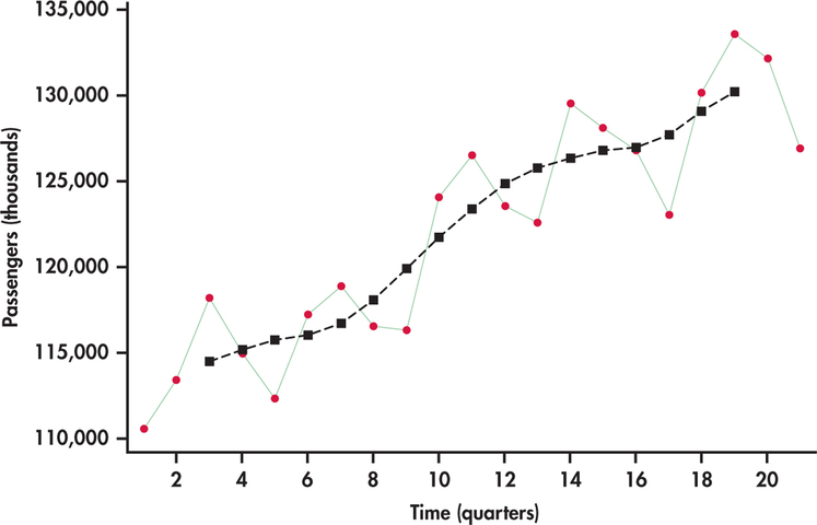
It can also be used to make predictions when the trend of the series has a constant mean.
A moving average is an arithmetic mean that is characterized by the fact that it takes a value for each moment in time and that not all the available sample observations are included in its calculation.
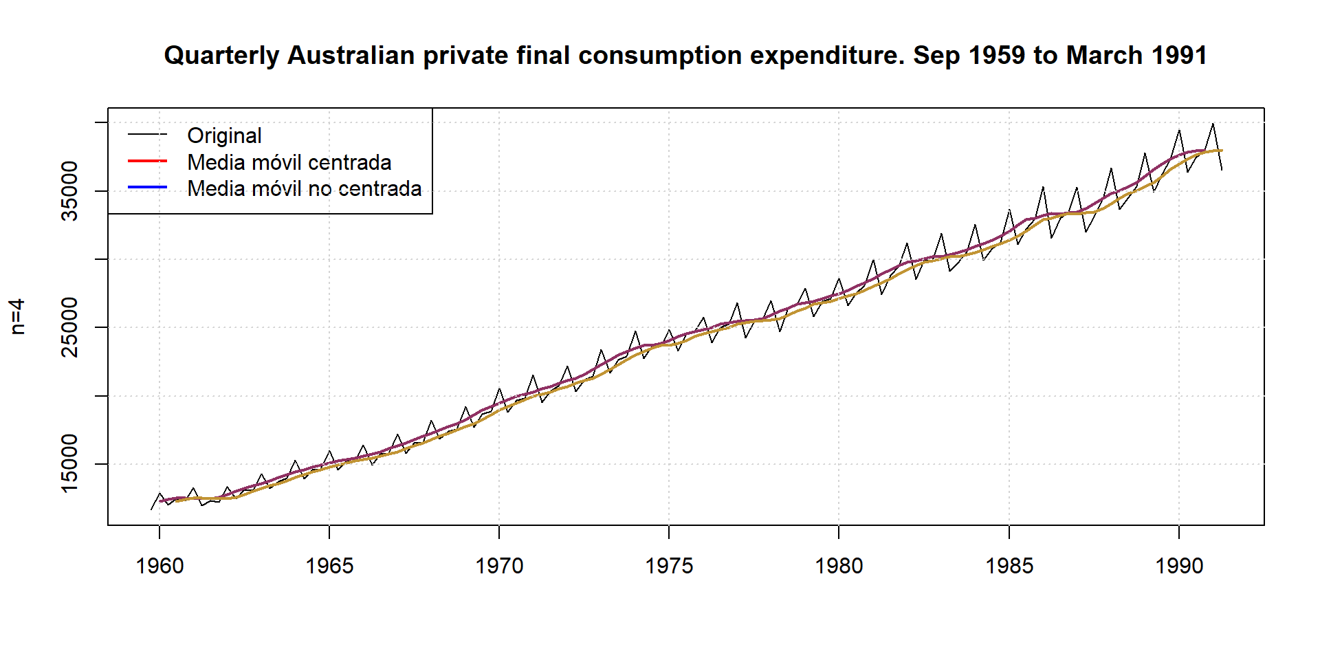
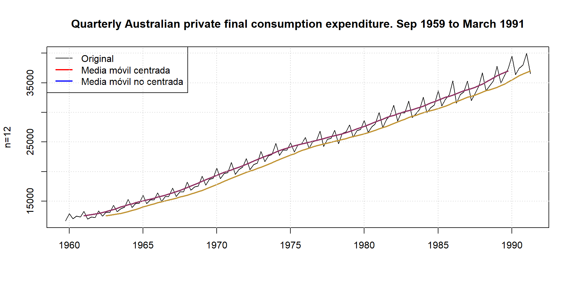
Of the different types of moving averages that can be constructed, we are going to refer to two types: centered moving averages and asymmetric moving averages. The first type is used for trend representation, while the second type is used for prediction in models with constant mean.
###Centered moving averages
Centered moving averages are characterized by the fact that the number of observations that enter into their calculation is odd, each moving average being assigned to the central observation. Thus, a moving average centered on \(t\) of length \(2n+1\) is given by the following expression:
\[ MM(2n+1)_t=\dfrac{y_{t-n}+y_{t-n+1}+...+y_t+...+y_{t+n-1}+y_{t+n}}{2n+1} \]
As can be seen, the subscript assigned to the moving average, \(t\), is the same as that of the central observation, \(y_t\). Note also that, by construction, the moving averages corresponding to the \(n\) first and \(n\) last observations cannot be calculated.
16.1.1 Non-centered moving averages
In the case of asymmetric (non-centered) moving averages, each moving average is assigned to the period corresponding to the most advanced observation of all those involved in its calculation. Thus, the asymmetric moving average of \(n\) points associated to observation \(t\) will have the following expression:
\[ MMA(n)_t=\dfrac{y_{t-n+1}+y_{t-n+2}+...+Y_{t-1}+y_{t}}{n} \]
The use of moving averages implies the arbitrary choice of their length or order, i.e. the number of observations involved in the calculation of each moving average.
The longer the length, the better the irregularities of the series will be eliminated, since the more observations involved in its calculation, the more fluctuations of this type will be compensated, but on the contrary, the higher the information cost will be.
On the other hand, when the length is small, the moving average reflects more quickly the changes that may occur in the evolution of the series.
It is therefore advisable to balance these factors when deciding on the length of the moving average.