21 Non-Stationary Stochastic Processes
A stochastic process $ (Y_{t}right)$ is non-stationary when the statistical properties of at least one finite sequence $ Y_{t_{1}}}, Y_{t_{2}}, , Y_{t_{n}}(n ) $ of components of $ (Y_{t}right) $, are different from those of the sequence \(Y_{t_{1}+h}, Y_{t_{2}+h}, \ldots, Y_{t_{n}+h}\) for at least one integer \(h>0\).
Many time series cannot be considered to be generated by stationary stochastic processes (i.e., they are non-stationary series), because:
- they show some clear trend in their time evolution (so that they do not show affinity towards some constant value over time),
- because their dispersion is not constant, because they are seasonal, or for various combinations of these reasons
However, many non-stationary time series can be transformed in a suitable way to obtain stationary-looking series, which can be used as a starting point to build \(operatorname{ARMA}(p, q)\) models in practice.
To convert a non-stationary series into a stationary one, two types of transformations are usually employed in practice: a first type to stabilize its dispersion (i.e. to induce variance stationarity) and a second type to stabilize its level (i.e. to eliminate its trend or to induce mean stationarity).
21.0.1 Non-stationarity in Variance
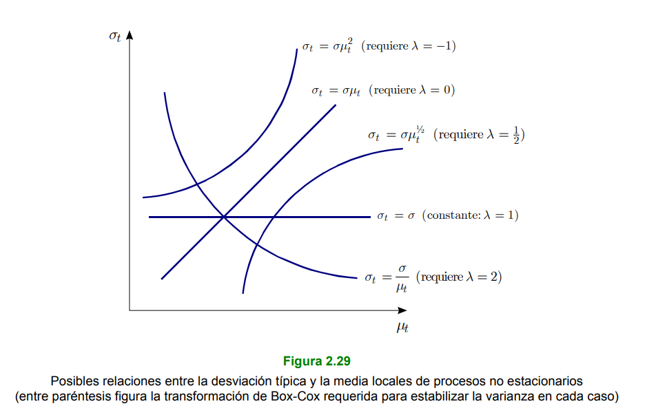
Let \(\left(Y_{t}\right)\) a non-stationary stochastic process such that
\[ \mu_{t} \equiv \mathrm{E}\left[Y_{t}\right] \, \text { and } \, \sigma_{t}^{2} \equiv \operatorname{Var}\left[Y_{t}\right] \] existen y dependen de \(t\) (por lo que no son constantes). Si
\[ \sigma_{t}^{2}=\sigma^{2} \times h\left(\mu_{t}\right)^{2} \]
where $ ^{2}>0 $ is a constant and $ h() $ is a real function such that $ h() $ for any value of $ {t}$, then a variance-stabilizing transformation of $ (Y{t}right) $ is any real function \(g(\cdot)\) such that $ g^{prime}()= $ for any value of $ _{t} . $
21.0.1.1 Dispersion Stabilization - Logarithmic Transformation
When the dispersion of a non-stationary time series $ Y_{t}(t=1, , N) $ is not constant because its local standard deviation is approximately proportional to its local level, the dispersion of the log-transformed series $ {t}=Y{t}(t=1, , N) $ is usually reasonably stable.
21.0.2 Non-stationarity in Mean
A stochastic process $ (Y_{t}right) $ is integrated of order $ d(d $ integer), or $ () $, if and only if the process $ (^{d} Y_{t}right) $ follows a $ (p, q) $ model that is stationary and invertible. In such a case, it is usually written
\[\left(Y_{t}\right) \sim \mathrm{I}(d)\].
21.0.2.1 Mean Level Stabilization (average) General - Regular Differentiation
The regular difference operator of order $ d(d .$ integer) is represented by the symbol \(\nabla^{d}\) \(\left(\right.\) sometimes \(\left.\Delta^{d}\right)\) and is defined as \(\nabla^{d} \equiv(1-B)^{d}\) (where \(B\) is the lad operator), so such that
\[ \nabla X_{t} \equiv X_{t}-X_{t-1}, \nabla^{2} X_{t} \equiv X_{t}-2 X_{t-1}+X_{t-2}, \ldots \]
where \(X_{t}\) is a variable (real or random) relative to a given time \(t\).
21.0.2.2 Deseasonalization - Seasonal Differentiation
The seasonal difference operator of period \(S\) and order \(D(D \geq 1\) integer) is represented by the symbol ${S}^{D} $ (sometimes $ . {S}^{D} )$ and is defined as $ _{S}^{D} (1-B^{S} )^{D} $ (where \(B\) is the delay operator), so that, in particular (when \(D=1\) ),
\[ \nabla_{S} X_{t} \equiv X_{t}-X_{t-S} \] where \(X_{t}\) is a variable (real or random) relative to a given time \(t\).