17.4 Operator \(B\)
17.4.1 Lag operator
Represented by \(B\) or \(L\), from Backshift operator o Lag operator.
\[ B Y_{t} = Y_{t-1s} \] where \(Y_{t}\) ia a time series at time \(t\)
- \(B\) indicates that the value at one instant is replaced by the value at the immediately preceding instant.
\[ B Y_{t} \equiv B(Y_{t-1}) \equiv B:Y_{t-1} \]
- A double application of \(B\) is denoted by:
\[ B^{2} Y_{t}=B\left(B Y_{t}\right)=B Y_{t-1}=Y_{t-2} \]
- In general,
\[ B^{d} Y_{t} = Y_{t-d} \]
17.4.2 Difference operator
Represented by the symbol \(\nabla\)
\[ \nabla Y_{t} = Y_{t} - Y_{t-1} \] where \(Y_{t}\) is a time series at time \(t\)
Examples:
\[ \begin{aligned} Y_{1}-Y_{0} &=\nabla Y_{1}\\ Y_{2}-Y_{1} &=\nabla Y_{2}\\ Y_{n}-Y_{n-1} &=\nabla Y_{n} \end{aligned} \] The regular difference of order d operator ( \(d\geq 1\) integer) is represented by \(\nabla^{d}\) (or \(\Delta^d\)) and denotes the successive application of \(\nabla:\)
\[ \nabla^{d} Y_{t} = (1-B)^d Y_{t} \]
For example:
\[ \begin{aligned} \nabla^{2} Y_{t} &=(1-B)^{2} Y_{t}=\left(1-2 B-B^{2}\right) Y_{t} \\ \nabla^{3} Y_{t} &=Y_{t}-3 B Y_{t}+3 B^{2} Y_{t}-B^{3} Y_{t} \end{aligned} \]
\(\nabla^{s}\) denotes the seasonal difference defined by:
\[ \nabla^{s} Y_{t} = (1-B^s) Y_{t} = Y_t - Y_{t-12} \]
17.4.3 Forward operator
Represented by the symbol \(B^-\) or \(F\)
\[ B^{-1}Y_{t} = Y_{t+1} \] where \(Y_{t}\) is a time series at time \(t\).
* F$ is the lag operator used in the inverse direction, i.e. \(d<0\), a new series will be ahead by \(d\) time units. * \(B^{-1}\) is the lead operator * In general, \[B^{-d} Y_{t} \equiv B^{-d}(Y_{t}) = Y_{t+d}\]
17.4.4 Properties of \(B\)
- The delay of a constant is a constant, \(c\):
\[ Bc=c \]
- Distributive property:
\[ \left(B^{i}+B^{j}\right) Y_{t}=B^{i} Y_{t}+B^{j} Y_{t}=Y_{t-i}-Y_{t-j} \]
- Associative property:
\[ \begin{aligned} B^{i} B^{j} X_{t}&=B^{i}\left(B^{j} Y_{t}\right)=B^{i} Y_{t-j}=Y_{t-i-j}\\ B^{i} B^{j} X_{t}&=B^{i+j} y_{t}, \text { y } \\ B^{0} X_{t}&=X_{t} \end{aligned} \]
- If \(|a| < 1,\)
\[ \left(1+a B+a^{2} B^{2}+a^{3} B^{3}+\ldots\right) Y_{t}=\frac{Y_{t}}{(1-a B)} \]
17.4.5 Equations in Difference
- A difference equation expresses the value of a variable as a function of its own lagged values, time and other variables.
- The \(B\) operator can be used to write compact difference equations:
\[ \begin{aligned} Y_{t} &=a_{0}+a_{1} Y_{t-1}+\ldots+a_{p} Y_{t-p}+\varepsilon_{t} \\ \left(1-a_{1} B-a_{2} B^{2}-\ldots-a_{p} B^{p}\right) Y_{t} &=a_{0}+\varepsilon_{t}\\ \Rightarrow A(B) X_{t}&=a_{0}+\varepsilon_{t} \end{aligned} \]
where \(A(B)\) can be viewed as a polynomial of the operator \(B.\)
- Another example:
\[ \begin{aligned} X_{t} &=a_{0}+a_{1} X_{t-1}+\ldots+a_{p} X_{t-p}+\varepsilon_{t}+\beta_{1} \varepsilon_{t-1}+\ldots+\beta_{q} \varepsilon_{t-q} \\ A(B) X_{t} &=a_{0}+M(B) \varepsilon_{t} \end{aligned} \]
The \(B\) operator can be used to solve equations in differences:
\[ Y_{t} = a_{0}+a_{1} Y_{t-1}+\varepsilon_{t} \\ Y_{t} = a_{0}+B Y_{t}+\varepsilon_{t} \\ Y_{t} = \frac{a_{0}+\varepsilon_{t}}{1-a_{1} B} \]
17.4.6 Example:
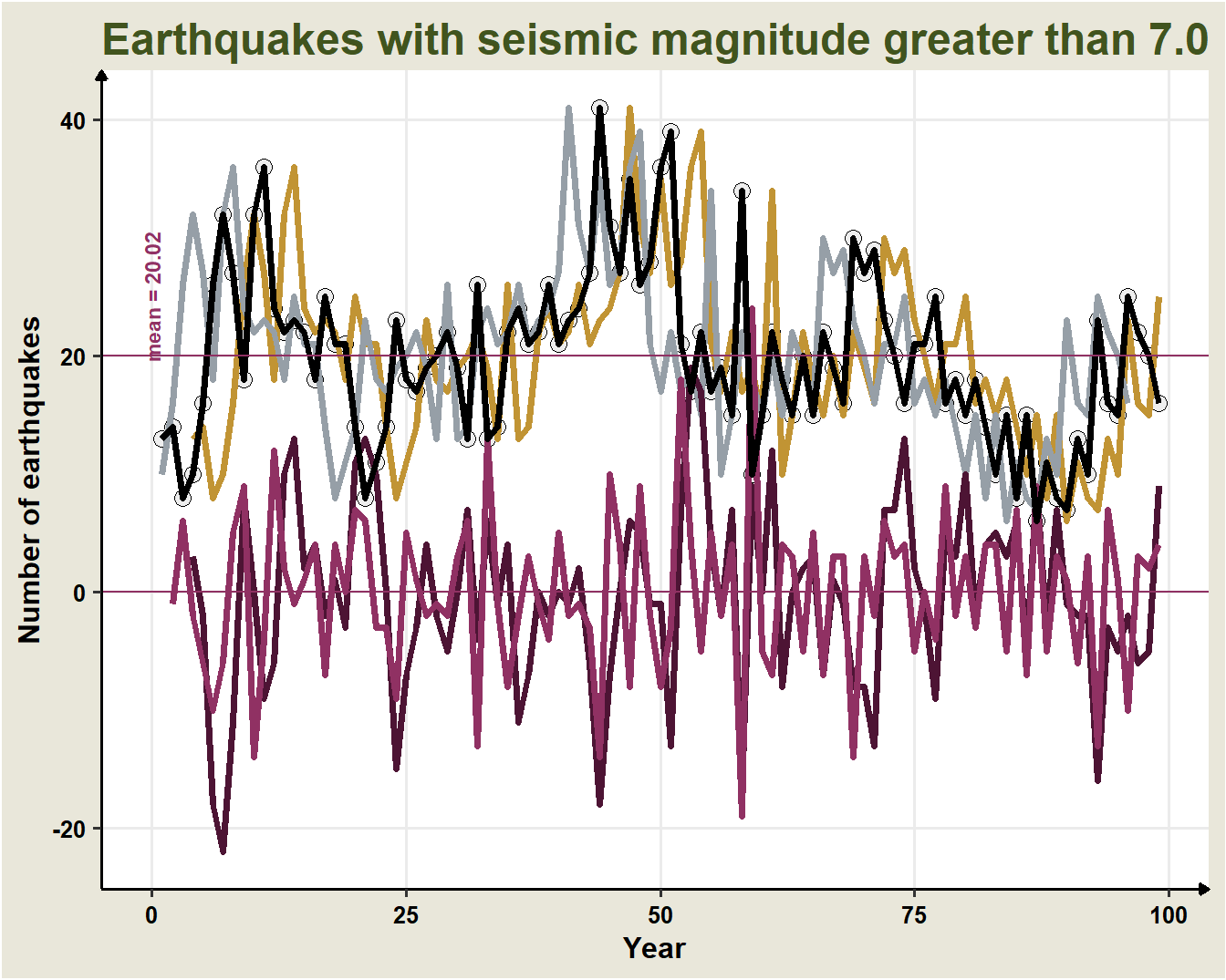
Applying the operator \(B\) to the series of earthquakes:
| \(t\) | \(Y_t\) | \(BY_{t}\) | \(B^3Y_{t}\) | \(B^{-1}Y_{t}\) | \(B^{-1}Y_{t}\) | \(\nabla Y_{t}\) | \(\nabla^{3}Y{t}\) |
|---|---|---|---|---|---|---|---|
| 1 | 13 | NA | NA | 14 | 10 | NA | NA |
| 2 | 14 | 13 | NA | 8 | 16 | -1 | NA |
| 3 | 8 | 14 | NA | 10 | 26 | 6 | NA |
| 4 | 10 | 8 | 13 | 16 | 32 | -2 | 3 |
| 5 | 16 | 10 | 14 | 26 | 27 | -6 | -2 |
| 6 | 26 | 16 | 8 | 32 | 18 | -10 | -18 |
| 7 | 32 | 26 | 10 | 27 | 32 | -6 | -22 |
| 8 | 27 | 32 | 16 | 18 | 36 | 5 | -11 |
| 9 | 18 | 27 | 26 | 32 | 24 | 9 | 8 |
| 10 | 32 | 18 | 32 | 36 | 22 | -14 | 0 |